The Binomial Distribution
The binomial distribution is a discrete probability distribution used to model the number of successes in a fixed number of repeated trials of the same experiment.

Conditions for a Binomial Model
A random variable \( X \) follows a binomial distribution if all of the following conditions are satisfied:
- There are a fixed number \( n \) of trials
- Each trial has only two possible outcomes: success or failure
- The probability of success \( p \) is the same for every trial
- Trials are independent
If these conditions are not met, a binomial model is not appropriate.
Notation
If a random variable \( X \) has a binomial distribution with parameters \( n \) and \( p \), this is written as
\( X \sim \mathrm{Bin}(n, p) \)
Probability Function
For \( X \sim \mathrm{Bin}(n, p) \), the probability that exactly \( x \) successes occur is
\( \mathrm{P}(X = x) = \mathrm{C}(n,x)\, p^x (1-p)^{n-x}, \quad x = 0,1,2,\dots,n \)
where \( \mathrm{C}(n,x) \) is the binomial coefficient.
Cumulative Binomial Probabilities
Cumulative probabilities involve sums of individual probabilities, for example
\( \mathrm{P}(X \leq k) = \sum_{x=0}^{k} \mathrm{P}(X=x) \)
These probabilities may be found:
- By direct calculation
- By using binomial probability tables
Tables are particularly useful when \( n \) is large.
Modelling and Appropriateness
When using a binomial distribution to model a real-world situation, students should:
- Clearly define what counts as a success
- Check that the probability of success remains constant
- Comment on whether independence of trials is reasonable
If these assumptions are unrealistic, the binomial distribution may not be appropriate.
Example :
A biased coin has a probability of landing heads equal to \( \mathrm{p} = 0.6 \). The coin is tossed 5 times.
Find the probability that exactly 3 heads are obtained.
▶️ Answer/Explanation
Let \( \mathrm{X} \sim \mathrm{Bin}(5, 0.6) \).
\( \mathrm{P}(X = 3) = \mathrm{C}(5,3)(0.6)^3(0.4)^2 \)
\( = 10 \times 0.216 \times 0.16 = 0.3456 \)
Conclusion: The probability is 0.3456.
Example :
A factory produces items, each of which has a probability of being defective equal to 0.02. A random sample of 10 items is selected.
Find the probability that at most one item is defective.
▶️ Answer/Explanation
Let \( \mathrm{X} \sim \mathrm{Bin}(10, 0.02) \), where a success represents a defective item.
We require
\( \mathrm{P}(X \leq 1) = \mathrm{P}(X = 0) + \mathrm{P}(X = 1) \)
\( \mathrm{P}(X = 0) = (0.98)^{10} \)
\( \mathrm{P}(X = 1) = \mathrm{C}(10,1)(0.02)(0.98)^9 \)
\( \mathrm{P}(X \leq 1) = 0.8171 + 0.1668 = 0.9839 \)
Conclusion: The probability is approximately 0.984.
Example :
A basketball player has a probability of 0.75 of scoring a free throw. She takes 8 independent free throws.
Find the probability that she scores at least 6 free throws. Comment on the suitability of a binomial model.
▶️ Answer/Explanation
Let \( \mathrm{X} \sim \mathrm{Bin}(8, 0.75) \).
Using the complement:
\( \mathrm{P}(X \geq 6) = 1 – \mathrm{P}(X \leq 5) \)
\( \mathrm{P}(X \leq 5) = \mathrm{P}(X=0)+\cdots+\mathrm{P}(X=5) \)
\( \mathrm{P}(X \geq 6) = 0.678 \) (from binomial tables)
Comment: The binomial model is appropriate because the number of trials is fixed, outcomes are success or failure, the probability of success is constant, and trials are independent.
Conclusion: The probability is approximately 0.678.
The Poisson Distribution
The Poisson distribution is a discrete probability distribution used to model the number of times an event occurs in a fixed interval of time, area, volume, or length, when the events occur randomly and independently.
Conditions for a Poisson Model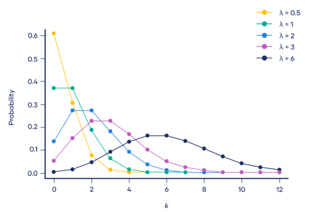
A Poisson distribution is appropriate if:
- Events occur independently of one another
- The average rate of occurrence is constant
- Two events cannot occur at exactly the same instant
- Events occur randomly in the given interval
If these assumptions are unrealistic, the Poisson model may not be appropriate.
Notation
If a random variable \( X \) follows a Poisson distribution with mean \( \lambda \), this is written as
\( X \sim \mathrm{Po}(\lambda) \)
Here, \( \lambda \) represents the mean number of events in the given interval.
Probability Function
For \( X \sim \mathrm{Po}(\lambda) \), the probability that exactly \( x \) events occur is given by
\( \mathrm{P}(X = x) = \dfrac{e^{-\lambda}\lambda^x}{x!}, \quad x = 0,1,2,\dots \)
This formula may be used directly. Derivation is not required.
Cumulative Poisson Probabilities
Cumulative probabilities are calculated by summing individual probabilities, for example
\( \mathrm{P}(X \leq k) = \sum_{x=0}^{k} \mathrm{P}(X=x) \)
These probabilities may be found:
- By direct calculation
- By using Poisson probability tables
Additive Property of the Poisson Distribution
If the number of events occurring in one unit of time follows
\( X \sim \mathrm{Po}(\lambda) \)
then the number of events occurring in \( t \) units of time follows
\( Y \sim \mathrm{Po}(t\lambda) \)
For example, if the number of arrivals per minute follows \( \mathrm{Po}(\lambda) \), then the number of arrivals per 5 minutes follows \( \mathrm{Po}(5\lambda) \).
Modelling and Appropriateness
When using a Poisson distribution to model a real-world situation, students should:
- Identify the interval clearly
- Interpret \( \lambda \) as the mean rate of occurrence
- Comment on whether independence and randomness are reasonable
If events cluster or occur regularly, the Poisson model may not be suitable.
Example :
The number of phone calls received by a call centre per minute follows a Poisson distribution with mean 2 calls per minute.
Find the probability that exactly 3 calls are received in a given minute.
▶️ Answer/Explanation
Let \( X \sim \mathrm{Po}(2) \).
\( \mathrm{P}(X = 3) = \dfrac{e^{-2} 2^3}{3!} \)
\( = \dfrac{e^{-2} \times 8}{6} = 0.1804 \)
Conclusion: The probability is approximately 0.180.
Example :
The number of accidents occurring at a junction per week follows a Poisson distribution with mean 1.5.
Find the probability that at most one accident occurs in a given week.
▶️ Answer/Explanation
Let \( X \sim \mathrm{Po}(1.5) \).
We require
\( \mathrm{P}(X \leq 1) = \mathrm{P}(X = 0) + \mathrm{P}(X = 1) \)
\( \mathrm{P}(X = 0) = e^{-1.5} \)
\( \mathrm{P}(X = 1) = e^{-1.5}(1.5) \)
\( \mathrm{P}(X \leq 1) = e^{-1.5}(1 + 1.5) = 0.5578 \)
Conclusion: The probability is approximately 0.558.
Example :
The number of emails received by an office follows a Poisson distribution with mean 4 per hour.
Find the probability that fewer than 3 emails are received in a 30-minute period.
▶️ Answer/Explanation
Mean per hour is 4, so mean per 30 minutes is
\( \lambda = 4 \times \dfrac{1}{2} = 2 \)
Let \( X \sim \mathrm{Po}(2) \).
We require
\( \mathrm{P}(X < 3) = \mathrm{P}(X = 0) + \mathrm{P}(X = 1) + \mathrm{P}(X = 2) \)
\( = e^{-2}\left(1 + 2 + \dfrac{2^2}{2}\right) = 0.6767 \)
Conclusion: The probability is approximately 0.677.