Edexcel IAL - Statistics 2- 2.2 Probability Density and Distribution Functions- Study notes  - New syllabus

The Probability Density Function and the Cumulative Distribution Function

For a continuous random variable, probabilities are described using a probability density function (pdf) and a cumulative distribution function (cdf).

Probability Density Function (pdf)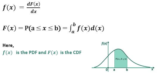

A probability density function, denoted by \( f(x) \), satisfies the following conditions:

\( f(x) \geq 0 \) for all \( x \)

The total area under the graph of \( f(x) \) is 1

\( \displaystyle \int_{-\infty}^{\infty} f(x)\,\mathrm{d}x = 1 \)

The function \( f(x) \) itself does not give probabilities. Probabilities are obtained by finding areas under the curve.

Using the Probability Density Function

For a continuous random variable \( X \) with pdf \( f(x) \), the probability that \( X \) lies in an interval is given by

\( \mathrm{P}(a < X \leq b) = \displaystyle \int_{a}^{b} f(x)\,\mathrm{d}x \)

Since \( \mathrm{P}(X=a)=0 \), the probabilities

• \( \mathrm{P}(a < X \leq b) \)
• \( \mathrm{P}(a \leq X < b) \)
• \( \mathrm{P}(a \leq X \leq b) \)

are all equal.

Cumulative Distribution Function (cdf)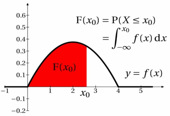 

The cumulative distribution function of a continuous random variable \( X \) is defined by

\( \mathrm{F}(x_0) = \mathrm{P}(X \leq x_0) = \displaystyle \int_{-\infty}^{x_0} f(x)\,\mathrm{d}x \)

The cdf gives the probability that the random variable takes a value less than or equal to a given number.

Relationship Between pdf and cdf

For a continuous random variable:

• The cdf is obtained by integrating the pdf
• The pdf is the derivative of the cdf, where it exists
• \( \mathrm{f}(x) = \dfrac{\mathrm{d}}{\mathrm{d}x}\,\mathrm{F}(x) \)

Form of the Probability Density Function

In this syllabus, probability density functions will be restricted to:

• Simple polynomial functions
• Piecewise-defined functions

These forms allow probabilities and cumulative distribution functions to be found using straightforward integration.