Edexcel IAL - Statistics 2- 3.1 Continuous Uniform Distribution- Study notes  - New syllabus

The Continuous Uniform (Rectangular) Distribution

The continuous uniform distribution, also called the rectangular distribution, models a situation where a continuous random variable is equally likely to take any value within a fixed interval.

This distribution is commonly used when there is no reason to believe that any value in the interval is more likely than another.

Definition

Let \( X \) be a continuous random variable uniformly distributed on the interval \( [a,b] \), where \( a < b \).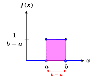

\( X \sim \mathrm{U}(a,b) \)

Probability Density Function

The probability density function of \( X \sim \mathrm{U}(a,b) \) is

\( \mathrm{f}(x) = \begin{cases} \dfrac{1}{b-a}, & a \leq x \leq b \\ 0, & \text{otherwise} \end{cases} \)

This constant height gives the distribution its rectangular shape.

Cumulative Distribution Function

The cumulative distribution function is found by integrating the pdf.

For \( x \in [a,b] \):

\( \mathrm{F}(x) = \displaystyle \int_{a}^{x} \dfrac{1}{b-a}\,\mathrm{d}t = \dfrac{x-a}{b-a} \)

Hence, the full cdf is

\( \mathrm{F}(x) = \begin{cases} 0, & x < a \\ \dfrac{x-a}{b-a}, & a \leq x \leq b \\ 1, & x > b \end{cases} \)

Derivation of the Mean

The mean of a continuous random variable is given by

\( \mathrm{E}(X) = \displaystyle \int_{a}^{b} x\,\mathrm{f}(x)\,\mathrm{d}x \)

For the uniform distribution:

\( \mathrm{E}(X) = \dfrac{1}{b-a} \displaystyle \int_{a}^{b} x\,\mathrm{d}x \)

\( = \dfrac{1}{b-a} \left[ \dfrac{x^2}{2} \right]_{a}^{b} = \dfrac{b^2 – a^2}{2(b-a)} \)

\( = \dfrac{a+b}{2} \)

Hence, the mean is the midpoint of the interval.

Derivation of the Variance

First find \( \mathrm{E}(X^2) \):

\( \mathrm{E}(X^2) = \dfrac{1}{b-a} \displaystyle \int_{a}^{b} x^2\,\mathrm{d}x \)

\( = \dfrac{1}{b-a} \left[ \dfrac{x^3}{3} \right]_{a}^{b} = \dfrac{b^3 – a^3}{3(b-a)} \)

The variance is

\( \mathrm{Var}(X) = \mathrm{E}(X^2) – [\mathrm{E}(X)]^2 \)

\( = \dfrac{b^3 – a^3}{3(b-a)} – \left(\dfrac{a+b}{2}\right)^2 \)

\( = \dfrac{(b-a)^2}{12} \)

Hence, the variance depends only on the width of the interval.

Summary of Results

Distribution: \( X \sim \mathrm{U}(a,b) \)

Mean: \( \dfrac{a+b}{2} \)

Variance: \( \dfrac{(b-a)^2}{12} \)

CDF: \( \mathrm{F}(x) = \dfrac{x-a}{b-a} \) for \( a \leq x \leq b \)