Normal Approximation to the Binomial and Poisson Distributions
In many practical situations, the Normal distribution can be used as an approximation to both the binomial and the Poisson distributions. This is particularly useful when exact calculations are difficult.
When using a Normal approximation, a continuity correction must be applied.
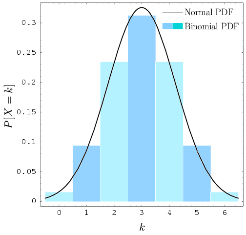
Normal Approximation to the Binomial Distribution
A binomial random variable \( X \sim \mathrm{Bin}(n,p) \) may be approximated by a Normal distribution if: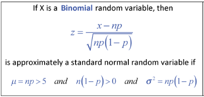
\( n \) is large
Neither \( p \) nor \( 1-p \) is close to 0
A commonly used guideline is:
\( np \geq 5 \quad \text{and} \quad n(1-p) \geq 5 \)
Under these conditions:
\( X \approx \mathrm{N}\!\left(np,\; np(1-p)\right) \)
Normal Approximation to the Poisson Distribution
A Poisson random variable \( X \sim \mathrm{Po}(\lambda) \) may be approximated by a Normal distribution when: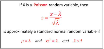
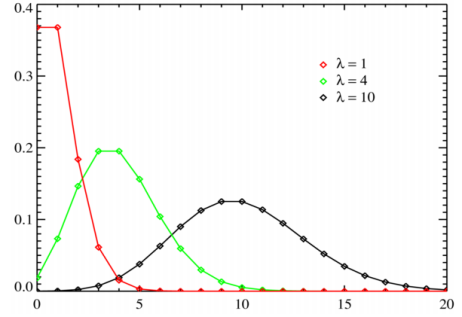
The mean \( \lambda \) is large
A common guideline is:
\( \lambda \geq 10 \)
In this case:
\( X \approx \mathrm{N}(\lambda,\; \lambda) \)
The Continuity Correction
The binomial and Poisson distributions are discrete, whereas the Normal distribution is continuous.
To improve accuracy, a continuity correction is applied when approximating discrete probabilities using the Normal distribution.
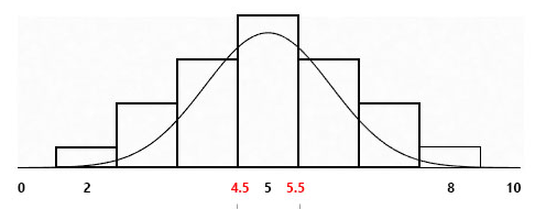
This involves adjusting the discrete value by \( \pm 0.5 \).
Continuity Correction Rules
| Discrete Probability | Normal Approximation |
|---|---|
| \( \mathrm{P}(X = k) \) | \( \mathrm{P}(k-0.5 < X < k+0.5) \) |
| \( \mathrm{P}(X \leq k) \) | \( \mathrm{P}(X < k+0.5) \) |
| \( \mathrm{P}(X \geq k) \) | \( \mathrm{P}(X > k-0.5) \) |
Standardisation
After applying the continuity correction, probabilities are found by standardising:
\( Z = \dfrac{X – \mu}{\sigma} \)
and using Normal distribution tables.
Examination Points
- Always check that the approximation conditions are satisfied
- State the mean and variance clearly before standardising
- Always apply the continuity correction
Example :
A random variable \( X \) follows a binomial distribution with parameters \( n = 100 \) and \( p = 0.4 \).
Use a Normal approximation to find \( \mathrm{P}(X \leq 45) \).
▶️ Answer/Explanation
Check conditions:
\( np = 40 \geq 5 \), \( n(1-p) = 60 \geq 5 \) ✓
Mean and variance:
\( \mu = np = 40,\quad \sigma^2 = np(1-p) = 24 \Rightarrow \sigma = \sqrt{24} \)
Apply continuity correction:
\( \mathrm{P}(X \leq 45) \approx \mathrm{P}(X < 45.5) \)
Standardise:
\( Z = \dfrac{45.5 – 40}{\sqrt{24}} = 1.12 \)
From Normal tables: \( \mathrm{P}(Z < 1.12) = 0.8686 \)
Conclusion: \( \mathrm{P}(X \leq 45) \approx 0.869 \).
Example :
The number of calls received by a call centre per hour follows a Poisson distribution with mean 25.
Use a Normal approximation to find \( \mathrm{P}(X \geq 30) \).
▶️ Answer/Explanation
Since \( \lambda = 25 \geq 10 \), the Normal approximation is appropriate.
Mean and variance:
\( \mu = 25,\quad \sigma^2 = 25 \Rightarrow \sigma = 5 \)
Apply continuity correction:
\( \mathrm{P}(X \geq 30) \approx \mathrm{P}(X > 29.5) \)
Standardise:
\( Z = \dfrac{29.5 – 25}{5} = 0.9 \)
\( \mathrm{P}(Z > 0.9) = 0.1841 \)
Conclusion: \( \mathrm{P}(X \geq 30) \approx 0.184 \).
Example:
A fair coin is tossed 200 times. Use a Normal approximation to find the probability that the number of heads is between 90 and 110 inclusive.
▶️ Answer/Explanation
Let \( X \sim \mathrm{Bin}(200, 0.5) \).
Mean and variance:
\( \mu = 100,\quad \sigma^2 = 50 \Rightarrow \sigma = \sqrt{50} \)
Apply continuity correction:
\( \mathrm{P}(90 \leq X \leq 110) \approx \mathrm{P}(89.5 < X < 110.5) \)
Standardise:
\( Z_1 = \dfrac{89.5 – 100}{\sqrt{50}} = -1.48,\quad Z_2 = \dfrac{110.5 – 100}{\sqrt{50}} = 1.48 \)
\( \mathrm{P}(-1.48 < Z < 1.48) = 0.8616 \)
Conclusion: The required probability is approximately 0.862.