Critical Region and Test Statistic
In a hypothesis test, decisions are made by comparing a calculated value with a pre-defined set of values known as the critical region. This comparison is based on a carefully chosen test statistic.
Test Statistic
A test statistic is a numerical value calculated from sample data that is used to decide whether to reject the null hypothesis.
It summarises the sample information relevant to the hypothesis being tested.
Examples of Test Statistics
- Sample mean \( \bar{x} \)
- Sample proportion
- Number of successes \( X \) in a binomial test
- Standardised Normal variable \( Z \)
The choice of test statistic depends on:
- The population distribution assumed under \( \mathrm{H_0} \)
- The parameter being tested
Critical Region
The critical region is the set of values of the test statistic for which the null hypothesis \( \mathrm{H_0} \) is rejected.
It is determined before the data are analysed, using the chosen significance level.
Significance Level
The significance level, usually denoted by \( \alpha \), is the probability of rejecting \( \mathrm{H_0} \) when it is actually true.
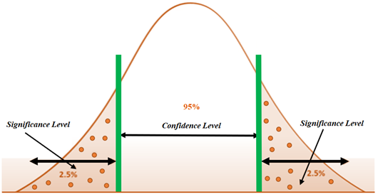
Common values: 10%, 5%, 1%
The critical region is chosen so that:
\( \mathrm{P}(\text{test statistic lies in critical region} \mid \mathrm{H_0}) = \alpha \)
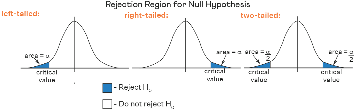
Types of Critical Regions
One-tailed Test
Used when the alternative hypothesis is directional.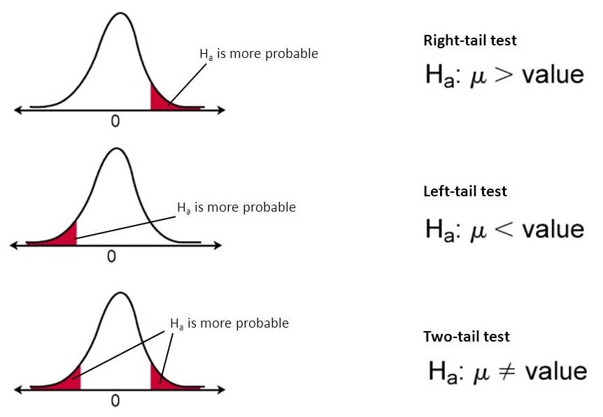
- Upper-tailed: reject \( \mathrm{H_0} \) for large values of the test statistic
- Lower-tailed: reject \( \mathrm{H_0} \) for small values of the test statistic
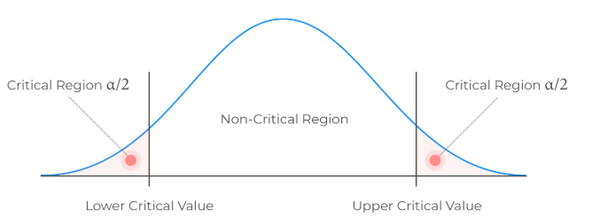
Two-tailed Test
Used when the alternative hypothesis is non-directional.
Critical regions lie in both tails of the distribution
Using the Test Statistic and Critical Region
The hypothesis test procedure is:
- State \( \mathrm{H_0} \) and \( \mathrm{H_1} \)
- Choose an appropriate test statistic
- Determine the critical region using the significance level
- Calculate the value of the test statistic from the sample
- Compare with the critical region and make a decision
Interpretation
If the test statistic lies in the critical region, the result is said to be statistically significant and \( \mathrm{H_0} \) is rejected.
If it does not lie in the critical region, there is insufficient evidence to reject \( \mathrm{H_0} \).
Key Points
- Always define the test statistic clearly
- State the critical region explicitly
- Use correct decision language
Example :
A coin is claimed to be fair. It is tossed 20 times and heads occur 15 times.
Test this claim at the 5% significance level.
▶️ Answer/Explanation
Let \( X \) be the number of heads.
Hypotheses:
\( \mathrm{H_0}:\; p = 0.5 \)
\( \mathrm{H_1}:\; p \neq 0.5 \)
Under \( \mathrm{H_0} \),
\( X \sim \mathrm{Bin}(20, 0.5) \)
From binomial tables:
\( \mathrm{P}(X \geq 15) = 0.0207 \)
Hence the critical region is:
\( X \geq 15 \) or \( X \leq 5 \)
Since the observed value is 15, it lies in the critical region.
Conclusion: Reject \( \mathrm{H_0} \). There is evidence that the coin is not fair.
Example :
The number of emails received per hour is modelled by a Poisson distribution with mean 4. In one hour, 9 emails are received.
Test the model at the 5% significance level.
▶️ Answer/Explanation
Let \( X \) be the number of emails in one hour.
Hypotheses:
\( \mathrm{H_0}:\; \lambda = 4 \)
\( \mathrm{H_1}:\; \lambda > 4 \)
Under \( \mathrm{H_0} \),
\( X \sim \mathrm{Po}(4) \)
From Poisson tables:
\( \mathrm{P}(X \geq 9) = 0.021 \)
Hence the critical region is:
\( X \geq 9 \)
The observed value lies in the critical region.
Conclusion: Reject \( \mathrm{H_0} \). The Poisson model with mean 4 may no longer be appropriate.
Example :
A population is normally distributed with known standard deviation 6. A random sample of 36 observations has mean 52.
Test the claim that the population mean is 50 at the 5% significance level.
▶️ Answer/Explanation
Hypotheses:
\( \mathrm{H_0}:\; \mu = 50 \)
\( \mathrm{H_1}:\; \mu \neq 50 \)
Test statistic:
\( Z = \dfrac{52 – 50}{6/\sqrt{36}} = 2 \)
Critical values for a two-tailed test at 5%:
\( Z = \pm 1.96 \)
Critical region:
\( Z < -1.96 \) or \( Z > 1.96 \)
Since \( Z = 2 \) lies in the critical region, the result is significant.
Conclusion: Reject \( \mathrm{H_0} \). There is evidence that the population mean differs from 50.