Hypothesis Tests for the Binomial Parameter \( \mathrm{p} \) and the Mean of a Poisson Distribution
Hypothesis testing can be used to assess whether observed data are consistent with an assumed value of a parameter in a binomial or Poisson model.
In this section, tests are carried out using:
- Exact probabilities from tables or calculation
- Normal approximations where appropriate
Binomial Hypothesis Test for the Parameter \( \mathrm{p} \)
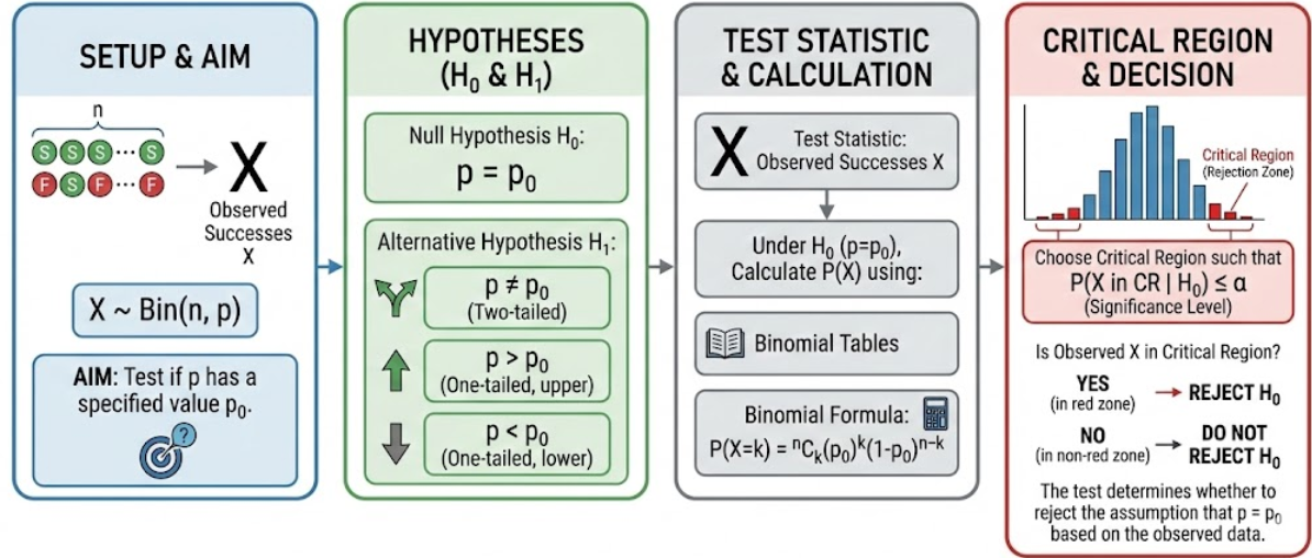
Let \( X \) be the number of successes in \( n \) trials, where
\( X \sim \mathrm{Bin}(n,p) \)
The aim is to test whether the probability of success \( p \) has a specified value.
Hypotheses
Typical hypotheses are:
Null hypothesis: \( \mathrm{H_0}:\; p = p_0 \)
Alternative hypothesis: \( \mathrm{H_1}:\; p \neq p_0 \), \( p > p_0 \), or \( p < p_0 \)
Test Statistic
The test statistic is:
The observed number of successes \( X \)
Under \( \mathrm{H_0} \), probabilities are calculated using:
- Binomial tables
- Direct calculation using the binomial formula
Critical Region
The critical region is chosen so that:
\( \mathrm{P}(X \text{ in critical region} \mid \mathrm{H_0}) \leq \alpha \)
If the observed value of \( X \) lies in the critical region, \( \mathrm{H_0} \) is rejected.
Normal Approximation for Binomial Tests
When \( n \) is large and:
\( np \geq 5 \quad \text{and} \quad n(1-p) \geq 5 \)
the binomial distribution may be approximated by a Normal distribution:
\( X \approx \mathrm{N}(np,\; np(1-p)) \)
A continuity correction must be applied.
Poisson Hypothesis Test for the Mean \( \mathrm{\lambda} \)
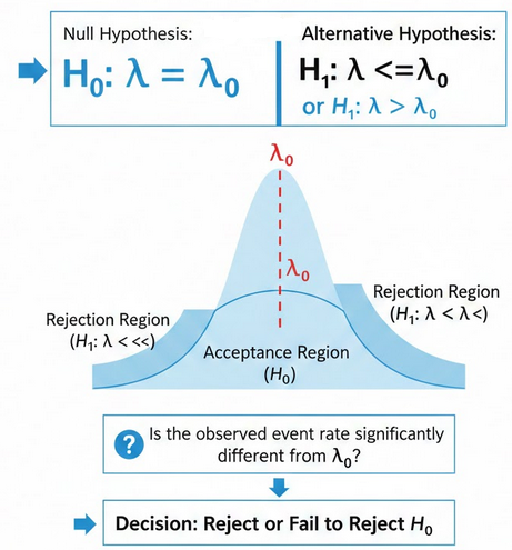
Let \( X \) be the number of events occurring in a fixed interval, where
\( X \sim \mathrm{Po}(\lambda) \)
The test examines whether the mean rate \( \lambda \) has a specified value.
Hypotheses
Typical hypotheses are:
Null hypothesis: \( \mathrm{H_0}:\; \lambda = \lambda_0 \)
Alternative hypothesis: \( \mathrm{H_1}:\; \lambda \neq \lambda_0 \), \( \lambda > \lambda_0 \), or \( \lambda < \lambda_0 \)
Test Statistic
The test statistic is:
The observed number of events \( X \)
Probabilities are obtained using:
- Poisson tables
- Direct calculation
Decision Rule
If the observed value lies in the critical region, the null hypothesis is rejected.
Otherwise, there is insufficient evidence to reject the null hypothesis.
Key Points
- Clearly state \( \mathrm{H_0} \) and \( \mathrm{H_1} \)
- Identify the correct distribution under \( \mathrm{H_0} \)
- Use tables or approximations correctly
- Apply a continuity correction where required
Example :
A factory claims that the probability a bulb is defective is \( 0.08 \). A random sample of 40 bulbs contains 6 defectives.
Test this claim at the 5% significance level.
▶️ Answer/Explanation
Let \( X \) be the number of defective bulbs.
Hypotheses:
\( \mathrm{H_0}:\; p = 0.08 \)
\( \mathrm{H_1}:\; p > 0.08 \)
Under \( \mathrm{H_0} \):
\( X \sim \mathrm{Bin}(40, 0.08) \)
Using binomial tables:
\( \mathrm{P}(X \geq 6) = 0.041 \)
Since \( 0.041 < 0.05 \), the result is significant.
Conclusion: Reject \( \mathrm{H_0} \). There is evidence that the defect probability exceeds 0.08.
Example :
In a large town, it is believed that 60% of households recycle regularly. A random sample of 200 households finds that 104 recycle.
Test this belief at the 5% significance level.
▶️ Answer/Explanation
Let \( X \) be the number of households that recycle.
Hypotheses:
\( \mathrm{H_0}:\; p = 0.6 \)
\( \mathrm{H_1}:\; p \neq 0.6 \)
Check conditions:
\( np = 120 \geq 5 \), \( n(1-p) = 80 \geq 5 \)
Normal approximation:
\( \mu = np = 120,\quad \sigma = \sqrt{np(1-p)} = \sqrt{48} \)
Apply continuity correction:
\( \mathrm{P}(X \leq 104) \approx \mathrm{P}(X < 104.5) \)
Standardise:
\( Z = \dfrac{104.5 – 120}{\sqrt{48}} = -2.24 \)
\( \mathrm{P}(Z < -2.24) = 0.0125 \)
Two-tailed probability \( = 2 \times 0.0125 = 0.025 \).
Conclusion: Reject \( \mathrm{H_0} \). The recycling proportion differs from 0.6.
Example :
A helpdesk receives calls at an average rate of 3 per hour. In one hour, 7 calls are received.
Test whether the call rate has increased, using a 5% significance level.
▶️ Answer/Explanation
Let \( X \) be the number of calls in one hour.
Hypotheses:
\( \mathrm{H_0}:\; \lambda = 3 \)
\( \mathrm{H_1}:\; \lambda > 3 \)
Under \( \mathrm{H_0} \):
\( X \sim \mathrm{Po}(3) \)
Using Poisson tables:
\( \mathrm{P}(X \geq 7) = 1 – \mathrm{P}(X \leq 6) = 0.033 \)
Since \( 0.033 < 0.05 \), the result is significant.
Conclusion: Reject \( \mathrm{H_0} \). There is evidence that the mean call rate has increased.