Edexcel IAL - Statistics 3- 3.6 Central Limit Theorem and Large Sample Tests- Study notes  - New syllabus

Use of the Central Limit Theorem for Inference

In practice, population distributions are often not normal and the population variance may be unknown. The Central Limit Theorem (CLT) allows hypothesis tests and confidence intervals for the mean to be extended to these situations when the sample size is sufficiently large.

The Central Limit Theorem

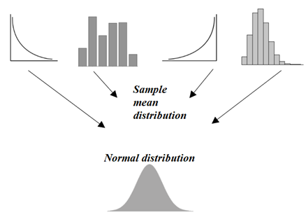
The Central Limit Theorem states that, for a random sample of size \( \mathrm{n} \) from any population with mean \( \mathrm{\mu} \) and finite variance \( \mathrm{\sigma^2} \), the distribution of the sample mean approaches a normal distribution as \( \mathrm{n} \) becomes large.

\( \mathrm{\bar{X} \approx N\!\left(\mu,\;\dfrac{\sigma^2}{n}\right)\ \text{for large } n} \)

In this syllabus, a sample size of about \( \mathrm{n \geq 30} \) is typically regarded as large.

Extension to Non-Normal Populations

Even if the population distribution is not normal:

The sample mean \( \mathrm{\bar{X}} \) is approximately normally distributed for large \( \mathrm{n} \)

Normal-based confidence intervals and hypothesis tests for the mean may be used

This allows inference for a wide range of real-world data.

Unknown Variance and Large Samples

When the population variance \( \mathrm{\sigma^2} \) is unknown, it is replaced by the sample variance \( \mathrm{S^2} \).

For large samples, the statistic

\( \mathrm{Z = \dfrac{\bar{X} – \mu}{S/\sqrt{n}}} \)

can be treated as having the standard normal distribution:

\( \mathrm{Z \sim N(0,1)} \)

A knowledge of the \( \mathrm{t} \)-distribution is not required for this syllabus.

Confidence Intervals Using CLT

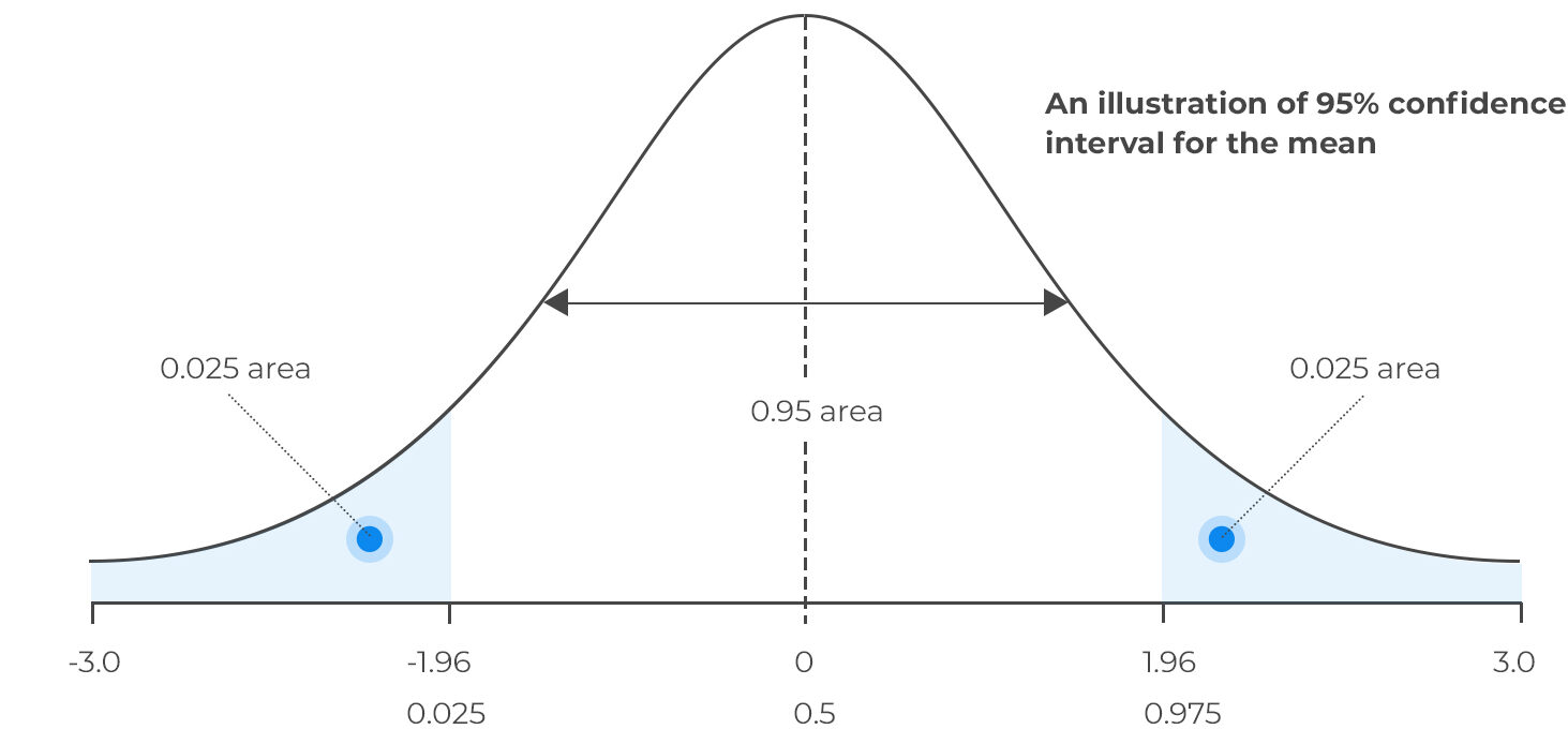
For large samples, an approximate \( \mathrm{(1-\alpha)\times100\%} \) confidence interval for the population mean is

\( \mathrm{\bar{X} \pm z_{\alpha/2}\dfrac{S}{\sqrt{n}}} \)

This interval is valid even when the population is not normal, provided the sample size is sufficiently large.

Hypothesis Tests Using CLT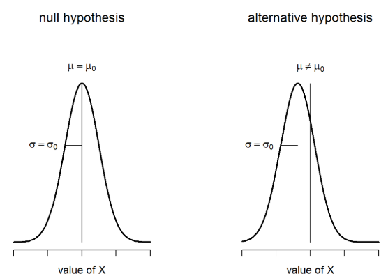

For testing

\( \mathrm{H_0:\mu = \mu_0} \)

the test statistic used is

\( \mathrm{Z = \dfrac{\bar{X} – \mu_0}{S/\sqrt{n}}} \)

Critical values and p-values are obtained from the standard normal distribution.

Conditions for Valid Use

• The sample is random and observations are independent
• The sample size is sufficiently large
• The population variance is finite

Points to Remember

• CLT allows inference for non-normal populations
• Large samples justify use of the normal distribution
• Unknown variance can be replaced by \( \mathrm{S^2} \) for large \( \mathrm{n} \)
• No knowledge of the \( \mathrm{t} \)-distribution is required