Hypothesis Test for the Difference Between Two Means (Variances Known)
In many situations, interest lies in comparing the means of two populations. When both populations are normally distributed and their variances are known, a normal test can be used to test hypotheses about the difference between their means.
Assumptions
The following conditions must be satisfied:

- Both populations are normally distributed
- The population variances \( \mathrm{\sigma_x^2} \) and \( \mathrm{\sigma_y^2} \) are known
- The two samples are random and independent
Sample Means
Let:
\( \mathrm{\bar{X}} \) be the mean of a sample of size \( \mathrm{n_x} \) from population X
\( \mathrm{\bar{Y}} \) be the mean of a sample of size \( \mathrm{n_y} \) from population Y
The difference between the sample means is \( \mathrm{\bar{X} – \bar{Y}} \).
Hypotheses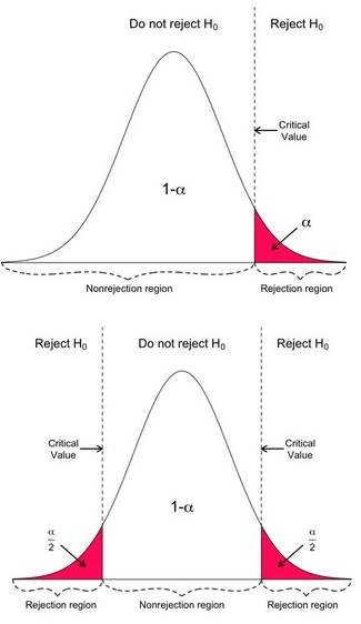
The null hypothesis usually takes the form:
\( \mathrm{H_0:\mu_x – \mu_y = d_0} \)
where \( \mathrm{d_0} \) is a specified value, often 0.
The alternative hypothesis may be:
Two-tailed: \( \mathrm{H_1:\mu_x – \mu_y \neq d_0} \)
Upper-tailed: \( \mathrm{H_1:\mu_x – \mu_y > d_0} \)
Lower-tailed: \( \mathrm{H_1:\mu_x – \mu_y < d_0} \)
Test Statistic
The test statistic used is
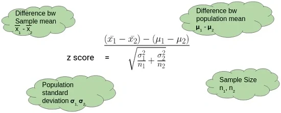
Under the null hypothesis,
\( \mathrm{Z \sim N(0,1)} \)
Decision Rule
Using the critical value approach:
Two-tailed 5% test: reject \( \mathrm{H_0} \) if \( \mathrm{|Z| > 1.96} \)
Upper-tailed 5% test: reject \( \mathrm{H_0} \) if \( \mathrm{Z > 1.645} \)
Lower-tailed 5% test: reject \( \mathrm{H_0} \) if \( \mathrm{Z < -1.645} \)
Alternatively, the p-value method may be used.
Interpretation
If \( \mathrm{H_0} \) is rejected, there is sufficient evidence of a difference between the population means
If \( \mathrm{H_0} \) is not rejected, there is insufficient evidence to conclude that the means differ
Key Points to Remember
- Both variances must be known
- The test statistic follows \( \mathrm{N(0,1)} \)
- This test compares population means, not sample means
Example :
Two independent normal populations X and Y have known standard deviations \( \mathrm{\sigma_x = 6} \) and \( \mathrm{\sigma_y = 8} \).
A sample of \( \mathrm{n_x = 36} \) from X has mean \( \mathrm{\bar{x} = 54} \), and a sample of \( \mathrm{n_y = 64} \) from Y has mean \( \mathrm{\bar{y} = 50} \).
Test at the 5% significance level whether the population means differ.
▶️ Answer/Explanation
Hypotheses
\( \mathrm{H_0:\mu_x – \mu_y = 0} \)
\( \mathrm{H_1:\mu_x – \mu_y \neq 0} \)
Test statistic
\( \mathrm{Z = \dfrac{(54-50)-0}{\sqrt{\dfrac{6^2}{36}+\dfrac{8^2}{64}}} = \dfrac{4}{\sqrt{1+1}} = \dfrac{4}{\sqrt{2}} = 2.83} \)
Decision
At 5%, reject \( \mathrm{H_0} \) if \( \mathrm{|Z|>1.96} \).
Conclusion
Since \( \mathrm{2.83>1.96} \), reject \( \mathrm{H_0} \). There is sufficient evidence that the population means differ.
Example :
The mean processing times of two machines X and Y are compared.
Known standard deviations are \( \mathrm{\sigma_x = 5} \) and \( \mathrm{\sigma_y = 4} \).
Samples of sizes \( \mathrm{n_x = 25} \) and \( \mathrm{n_y = 16} \) give means \( \mathrm{\bar{x} = 82} \) and \( \mathrm{\bar{y} = 80} \).
Test at the 5% level whether machine X has a greater mean processing time.
▶️ Answer/Explanation
Hypotheses
\( \mathrm{H_0:\mu_x – \mu_y = 0} \)
\( \mathrm{H_1:\mu_x – \mu_y > 0} \)
Test statistic
\( \mathrm{Z = \dfrac{(82-80)}{\sqrt{\dfrac{5^2}{25}+\dfrac{4^2}{16}}} = \dfrac{2}{\sqrt{1+1}} = \dfrac{2}{\sqrt{2}} = 1.41} \)
Decision
Upper-tailed 5% test: reject if \( \mathrm{Z>1.645} \).
Conclusion
Since \( \mathrm{1.41<1.645} \), do not reject \( \mathrm{H_0} \). There is insufficient evidence that machine X has a greater mean processing time.
Example :
Two independent normal populations have known variances \( \mathrm{\sigma_x^2 = 9} \) and \( \mathrm{\sigma_y^2 = 16} \).
A sample of \( \mathrm{n_x = 50} \) from X has mean \( \mathrm{\bar{x} = 20.6} \), and a sample of \( \mathrm{n_y = 40} \) from Y has mean \( \mathrm{\bar{y} = 21.4} \).
Test at the 1% significance level whether the population means are different.
▶️ Answer/Explanation
Hypotheses
\( \mathrm{H_0:\mu_x – \mu_y = 0} \)
\( \mathrm{H_1:\mu_x – \mu_y \neq 0} \)
Test statistic
\( \mathrm{Z = \dfrac{(20.6-21.4)}{\sqrt{\dfrac{9}{50}+\dfrac{16}{40}}} = \dfrac{-0.8}{\sqrt{0.18+0.4}} = \dfrac{-0.8}{0.76} = -1.05} \)
Decision
At 1% level, reject if \( \mathrm{|Z|>2.576} \).
Conclusion
Since \( \mathrm{|−1.05|<2.576} \), do not reject \( \mathrm{H_0} \). There is insufficient evidence at the 1% level to conclude that the population means differ.