Chi-squared Goodness of Fit Test
The chi-squared goodness of fit test is used to assess whether observed data are consistent with a specified theoretical distribution.
In this syllabus, the test is applied using the chi-squared test statistic, without lengthy calculations, to a range of common discrete and continuous distributions.
Null and Alternative Hypotheses
The hypotheses are:
Null hypothesis \( \mathrm{H_0} \): The data follow the specified distribution
Alternative hypothesis \( \mathrm{H_1} \): The data do not follow the specified distribution
The test checks whether any differences between observed and expected frequencies can reasonably be explained by random variation.
Observed and Expected Frequencies
For each category:
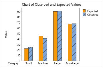
Observed frequency: \( \mathrm{O} \)
Expected frequency: \( \mathrm{E} \), calculated from the assumed distribution
Expected frequencies are usually found by multiplying the theoretical probability by the total number of observations.
Chi-squared Test Statistic
The chi-squared test statistic is
\( \mathrm{\chi^2 = \sum \dfrac{(O – E)^2}{E}} \)
This statistic measures the overall discrepancy between observed and expected frequencies.
Degrees of Freedom
The degrees of freedom are given by
\( \mathrm{df = k – 1 – m} \)
where:
\( \mathrm{k} \) = number of categories
\( \mathrm{m} \) = number of parameters estimated from the data
The critical value is obtained from chi-squared tables.
Decision Rule
Reject \( \mathrm{H_0} \) if the calculated \( \mathrm{\chi^2} \) value exceeds the critical value
Otherwise, do not reject \( \mathrm{H_0} \)
Distributions Used in This Test
Applications include:
- Discrete uniform distribution
- Binomial distribution
- Poisson distribution
- Normal distribution (grouped data)
- Continuous uniform (rectangular) distribution
Expected frequencies should generally be at least 5. Categories may be combined if necessary.
Key Points to Remember
- The test compares observed and expected frequencies
- Large values of \( \mathrm{\chi^2} \) indicate poor fit
- Lengthy calculations are not required in examinations
Example
A die is rolled 60 times. The observed frequencies of faces 1 to 6 are:
8, 11, 9, 10, 12, 10
Test at the 5% level whether the die is fair.
▶️ Answer/Explanation
Expected frequency for each face:
\( \mathrm{E = 60/6 = 10} \)
Calculate:
\( \mathrm{\chi^2 = \sum \dfrac{(O-E)^2}{E} = 1.0} \)
Degrees of freedom:
\( \mathrm{df = 6 – 1 = 5} \)
Critical value at 5%: 11.07
Conclusion: Since \( \mathrm{1.0 < 11.07} \), do not reject \( \mathrm{H_0} \). The data are consistent with a fair die.
Example
The number of calls received per hour is modelled by a Poisson distribution with mean 2.
Observed frequencies over 100 hours are:
0 calls: 14, 1 call: 28, 2 calls: 32, 3 or more calls: 26
Test the goodness of fit at the 5% level.
▶️ Answer/Explanation
Expected frequencies are calculated using Poisson probabilities.
Chi-squared statistic:
\( \mathrm{\chi^2 = 3.6} \)
Degrees of freedom:
\( \mathrm{df = 4 – 1 = 3} \)
Critical value at 5%: 7.81
Conclusion: Since \( \mathrm{3.6 < 7.81} \), do not reject \( \mathrm{H_0} \). The Poisson model is reasonable.
Example
Random numbers between 0 and 1 are grouped into five equal intervals. The observed frequencies are:
18, 21, 19, 22, 20
Test at the 5% level whether the data come from a continuous uniform distribution.
▶️ Answer/Explanation
Total observations: 100
Expected frequency per interval:
\( \mathrm{E = 100/5 = 20} \)
Chi-squared statistic:
\( \mathrm{\chi^2 = 0.5} \)
Degrees of freedom:
\( \mathrm{df = 5 – 1 = 4} \)
Critical value at 5%: 9.49
Conclusion: Since \( \mathrm{0.5 < 9.49} \), do not reject \( \mathrm{H_0} \). The data are consistent with a uniform distribution.