Price Elasticity of Supply (PES)
PES = Percentage change in quantity supplied ÷ Percentage change in price
Definition
Price elasticity of supply (PES) measures how responsive the quantity supplied of a good is to a change in its price.
\( \mathrm{PES = \dfrac{\%\ \Delta Q_s}{\%\ \Delta P}} \)
Explanation of the Formula
- \( \mathrm{\%\ \Delta Q_s} \) refers to the percentage change in quantity supplied.
- \( \mathrm{\%\ \Delta P} \) refers to the percentage change in price.
- PES shows how easily producers can respond to price changes.
Understanding PES
- If producers can quickly increase output when price rises → supply is elastic.
- If producers cannot easily change output → supply is inelastic.
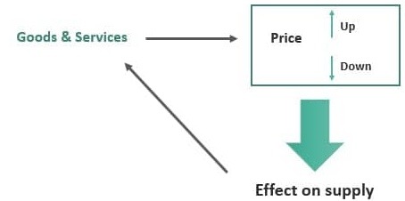
Price ↑ → Supply response depends on flexibility
Important Note
- Unlike PED, PES is usually positive.
- This is because price and quantity supplied have a direct relationship.
Key Ideas:
- PES measures producer responsiveness.
- It is a ratio of percentage changes.
- Depends on how easily firms can change production.
- Important for understanding market adjustments.
Example 1
Price increases by 10% and quantity supplied increases by 20%. Calculate PES.
▶️ Answer / Explanation
\( \mathrm{PES = \dfrac{20}{10} = 2} \)
Supply is elastic.
Example 2
At a price \( \mathrm{P_1 = \$50} \), producers supply \( \mathrm{Q_1 = 15} \) units.
At a price \( \mathrm{P_2 = \$100} \), producers supply \( \mathrm{Q_2 = 25} \) units.
Calculate the price elasticity of supply (PES).
▶️ Answer / Explanation
Step 1: Calculate percentage change in price
\( \mathrm{\%\ \Delta P = \dfrac{100 – 50}{50} \times 100 = 100\%} \)
Step 2: Calculate percentage change in quantity supplied
\( \mathrm{\%\ \Delta Q_s = \dfrac{25 – 15}{15} \times 100 = \dfrac{10}{15} \times 100 \approx 66.67\%} \)
Step 3: Apply PES formula
\( \mathrm{PES = \dfrac{\%\ \Delta Q_s}{\%\ \Delta P} = \dfrac{66.67}{100} = \dfrac{2}{3}} \)
Conclusion:
\( \mathrm{PES = \dfrac{2}{3} < 1} \), so supply is relatively inelastic.
Degrees of PES — Theoretical Range of Values
The value of price elasticity of supply (PES) shows the degree to which quantity supplied responds to a change in price.
\( \mathrm{PES = \dfrac{\%\ \Delta Q_s}{\%\ \Delta P}} \)
Theoretical Range of PES
\( \mathrm{0 \ \leq \ PES \ \leq \ \infty} \)
- PES is always positive because price and supply move in the same direction.
- Different values indicate different levels of responsiveness.
Degrees of PES
| Type of Supply | PES Value | Explanation |
|---|---|---|
Perfectly Inelastic | \( \mathrm{PES = 0} \) | No change in quantity supplied despite price change |
Relatively Inelastic | \( \mathrm{0 < PES < 1} \) | Small change in quantity supplied |
Unit Elastic | \( \mathrm{PES = 1} \) | Proportional change in quantity supplied |
Relatively Elastic | \( \mathrm{PES > 1} \) | Large change in quantity supplied |
Perfectly Elastic | \( \mathrm{PES = \infty} \) | Infinite response to price change |
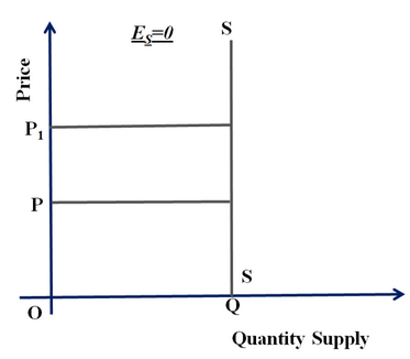
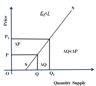
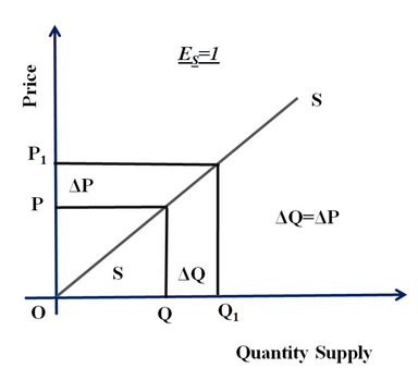
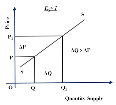
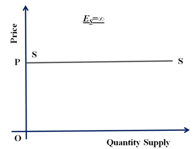
Diagram: Degrees of PES
- Perfectly inelastic → vertical supply curve
- Perfectly elastic → horizontal supply curve
- Elastic supply → flatter curve
- Inelastic supply → steeper curve
Economic Interpretation:
- High PES → firms can easily increase production.
- Low PES → firms face constraints in increasing output.
- Elasticity depends on production flexibility and time.
Key Ideas:
- PES ranges from 0 to infinity.
- Different values represent different supply responsiveness.
- Important for understanding producer behaviour.
- Helps analyse market adjustments to price changes.
Example 1
A good has \( \mathrm{PES = 0.2} \). Explain what this means.
▶️ Answer / Explanation
\( \mathrm{0 < PES < 1} \), so supply is relatively inelastic.
Quantity supplied responds only slightly to price changes.
Firms cannot easily increase production.
Example 2
Evaluate the meaning of perfectly elastic supply.
▶️ Answer / Explanation
Perfectly elastic supply means firms can supply any quantity at a given price.
The supply curve is horizontal.
Even a small price decrease reduces supply to zero.
This is a theoretical case, rarely seen in reality.