Question
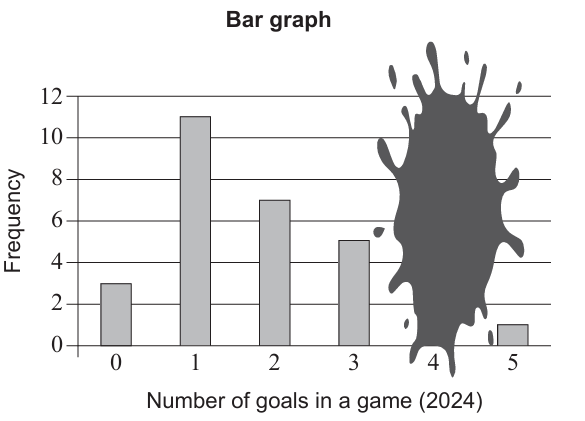
| Goals per match (\(2024\)) | Frequency |
|---|---|
| \(0\) | \(3\) |
| \(1\) | \(11\) |
| \(2\) | \(7\) |
| \(3\) | \(k\) |
| \(4\) | \(p\) |
| \(5\) | \(1\) |
(ii) Calculate the specific value of \(p\).
| Event | Description |
|---|---|
| \(A\) | Exactly \(2\) goals are scored in the match |
| \(B\) | More than \(1\) goal is scored in the match |
| \(C\) | At least \(2\) goals are scored in the match |
| \(D\) | \(0\) or \(1\) goal is scored in every match except this one |
| \(E\) | The score of \(0\) or \(1\) is not achieved in any match of the tournament |
Most-appropriate topic codes (IB Mathematics: Applications and Interpretation):
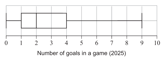
• SL 4.2: Production and understanding of box and whisker diagrams — part (c)
• SL 4.3: Measures of central tendency (mean/median) and dispersion (IQR/range) — parts (b), (c)
• SL 4.5: Concepts of sample space, probability, and complementary events — part (d)
• SL 4.6: Probability rules and calculation of combined events — parts (e), (f)
▶️ Answer/Explanation
(a)
From the bar graph provided in the context, the frequency for \(3\) goals is identified as \(5\).
\(\boxed{5}\)
(b)
(i) Mean \(= \frac{\text{Total Goals}}{\text{Total Matches}}\).
Total Matches \(= 3 + 11 + 7 + 5 + p + 1 = p + 27\).
Total Goals \(= (0 \times 3) + (1 \times 11) + (2 \times 7) + (3 \times 5) + (4 \times p) + (5 \times 1) = 45 + 4p\).
Given Mean \(= 2.2\), the equation is: \( \boxed{45 + 4p = 2.2(p + 27)} \)
(ii) Solving for \(p\):
\(45 + 4p = 2.2p + 59.4\)
\(1.8p = 14.4\)
\(p = 8\).
\(\boxed{8}\)
(c)
From the \(2024\) data: Total matches \(= 35\). Median is at the \(18^{th}\) position \(= 2\). \(Q_1\) is at the \(9^{th}\) position \(= 1\). \(Q_3\) is at the \(27^{th}\) position \(= 4\). \(\text{IQR} = 4 – 1 = 3\). Range \(= 5 – 0 = 5\).
From the \(2025\) box plot: Median \(= 2\), \(Q_1 = 1\), \(Q_3 = 4\), \(\text{IQR} = 3\), Range \(= 5\).
Consistent observations:
1. The median number of goals is \(2\) for both years.
2. The interquartile range (\(\text{IQR}\)) is \(3\) goals for both years.
(d)
Event \(F\) is “scoring \(0\) or \(1\) goal”. The complement \(F’\) is “not scoring \(0\) or \(1\) goal”, which is equivalent to “scoring at least \(2\) goals”.
Equivalent events from the list: \(B\) and \(C\).
\(\boxed{B, C}\)
(e)
Total matches in \(2024 = 35\). Initially, there are \(11\) matches with \(1\) goal.
After watching one match with \(1\) goal, \(34\) matches remain, of which \(10\) contain \(1\) goal.
Probability \(= \frac{10}{34} = \frac{5}{17}\).
\(\boxed{\frac{5}{17}}\)
(f)
Probability of first match having \(5\) goals \(= \frac{1}{35}\).
Probability of second match having \(0\) goals (given the first was different) \(= \frac{3}{34}\).
Total Probability \(= \frac{1}{35} \times \frac{3}{34} = \frac{3}{1190}\).
\(\boxed{\frac{3}{1190}}\)