Home / IB Mathematics AHL 5.16 first order differential equations AI HL Paper 2- Exam Style Questions

IB Mathematics AHL 5.16 first order differential equations AI HL Paper 2- Exam Style Questions- New Syllabus

Question

A market analyst is modeling the fluctuation in the price of a specific stock share, denoted by \(x\) dollars, at time \(t\) minutes after the release of a quarterly financial report. The model utilizes the following second-order differential equation:
\(\displaystyle \frac{d^2x}{dt^2} + 4 \frac{dx}{dt} + 3x = 0\)
This model can be expressed as a system of coupled first-order differential equations:
\(\displaystyle \frac{dx}{dt} = y,\quad \frac{dy}{dt} = -3x – 4y\)
(a) Determine the general solution for the displacement \(x\) in terms of \(t\).
At the moment the report is released (\(t = 0\)), the share value change is \(x = 0\) and the rate of change is \(\frac{dx}{dt} = -1\).
(b) (i) Derive a specific expression for \(x\) as a function of \(t\).
  (ii) Sketch the graph of \(x\) against \(t\) for the interval \(0 \leq t \leq 4\).
The analyst intends to purchase shares after the report’s release and sell them once the price recovers.
(c) (i) Based on your graph, identify the optimal time (in minutes) the analyst should wait before purchasing the shares to maximize potential profit.
  (ii) Calculate the theoretical maximum profit obtainable per share under this model.
To account for market volatility, a refined model is proposed:
\(\displaystyle \frac{d^2x}{dt^2} + 4 \frac{dx}{dt} + 3x = x \sin t\)
Applying the same initial conditions as previously stated:
(d) Use Euler’s method with a step size of \(h = 0.1\) to predict the value of \(x\) when \(t = 1\).

Most-appropriate topic codes:

AHL 5.17: Qualitative analysis of coupled differential equations using eigenvalues — part (a)
AHL 5.18: Solutions of second-order differential equations and phase portraits — part (b)
AHL 5.16: Numerical solution of coupled systems using Euler’s method — part (d)
SL 5.6: Local maximum and minimum points in context — part (c)
▶️ Answer/Explanation

(a)
The associated matrix is \( \begin{pmatrix} 0 & 1 \\ -3 & -4 \end{pmatrix} \).
Find eigenvalues: \(-\lambda(-4-\lambda) + 3 = 0 \Rightarrow \lambda^2 + 4\lambda + 3 = 0 \Rightarrow \lambda = -3, -1\).
General solution: \(x(t) = A e^{-3t} + B e^{-t}\).
\(\boxed{x = A e^{-3t} + B e^{-t}}\)

(b)(i)
Initial conditions: \(x(0) = 0\) ⇒ \(A + B = 0\) ⇒ \(B = -A\).
\( \frac{dx}{dt} = -3A e^{-3t} – B e^{-t} \).
At \(t = 0\), \(\frac{dx}{dt} = -1\) ⇒ \(-3A – B = -1\) ⇒ \(-3A + A = -1\) ⇒ \(-2A = -1\) ⇒ \(A = 0.5, B = -0.5\).
Thus \(x(t) = 0.5 e^{-3t} – 0.5 e^{-t}\).
\(\boxed{x = 0.5 e^{-3t} – 0.5 e^{-t}}\)

(b)(ii)

Graph of share value change over time
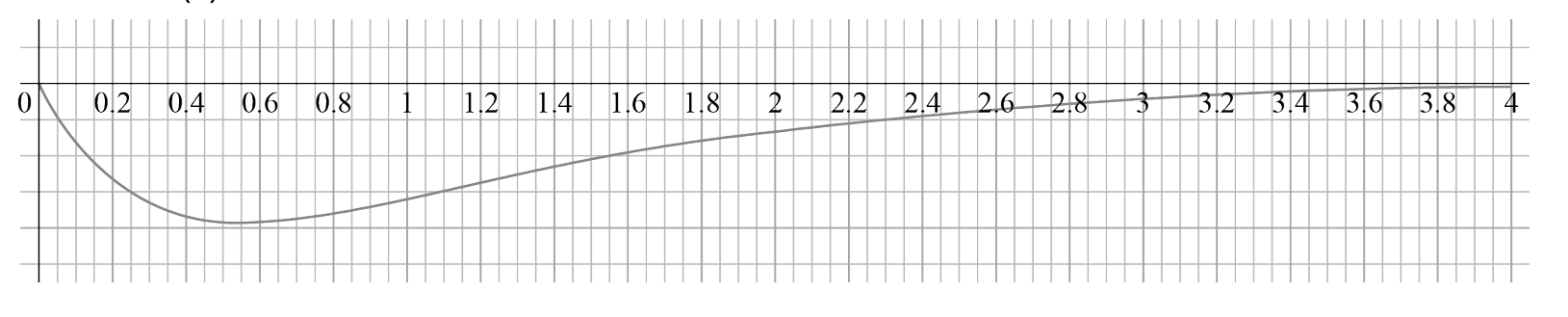
Sketch should show: starts at \(x=0\), decreases to a minimum near \(t \approx 0.55\), then increases asymptotically toward 0.

(c)(i)
The profit is maximized when \(x\) is minimized (buy low). From the graph, minimum occurs at \(t \approx 0.549\) minutes.
\(\boxed{0.549\ \text{minutes}}\)

(c)(ii)
Minimum value of \(x\) ≈ \(0.5 e^{-3(0.549)} – 0.5 e^{-0.549} \approx -0.192\).
Upper limit of profit per share ≈ \(0 – (-0.192) = 0.192\) dollars.
\(\boxed{0.192\ \text{dollars}}\)

(d)
Rewrite as coupled system:
\( \frac{dx}{dt} = y\), \( \frac{dy}{dt} = -4y – 3x + x \sin t\).
Initial: \(t_0 = 0, x_0 = 0, y_0 = -1\).
Step \(h = 0.1\):
\(x_{n+1} = x_n + 0.1 y_n\),
\(y_{n+1} = y_n + 0.1(-4y_n – 3x_n + x_n \sin t_n)\).
Iterate up to \(t = 1\) (10 steps):
After calculations, \(x_{10} \approx -0.172\).
\(\boxed{x(1) \approx -0.172}\)

Scroll to Top