Graphs Derived from Equations of Motion

Each equation of motion corresponds to a graphical representation of how one quantity changes with another. These graphs help visualize motion and are directly derived from:

• \( v = u + at \)
• \( s = ut + \dfrac{1}{2}at^2 \)
• \( v^2 = u^2 + 2as \)

1. Velocity–Time Graph from $v = u + at$

This equation shows that velocity increases linearly with time if acceleration is constant. It forms a straight line.

Graph Features:

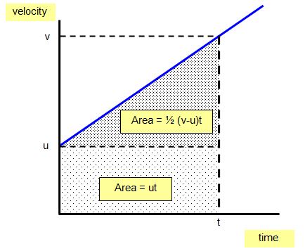
• Straight line with slope = acceleration \( a \)
• y-intercept = initial velocity \( u \)
• Area under graph = displacement \( s \)

From area under the graph:

Area = Trapezium = \( \dfrac{1}{2}(u + v)t = s \)

2. Displacement–Time Graph from $s = ut + \dfrac{1}{2}at^2$

This is a quadratic equation in \( t \), so the graph is a curve (a parabola).

Graph Features:

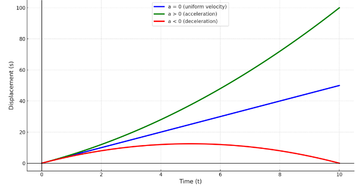
• If \( a = 0 \), the graph is a straight line (uniform velocity).
• If \( a > 0 \), the graph curves upwards (increasing velocity).
• If \( a < 0 \), the graph curves downwards (deceleration).

Shape is always a parabola when \( a \neq 0 \)

3. Velocity–Displacement Graph from $v^2 = u^2 + 2as$

Rewriting: \( v = \sqrt{u^2 + 2as} \)

This is a square root function. If we plot \( v \) vs \( s \), the graph is curved (non-linear).

Alternative: If we plot \( v^2 \) vs \( s \), the graph is linear.

Graph Features:

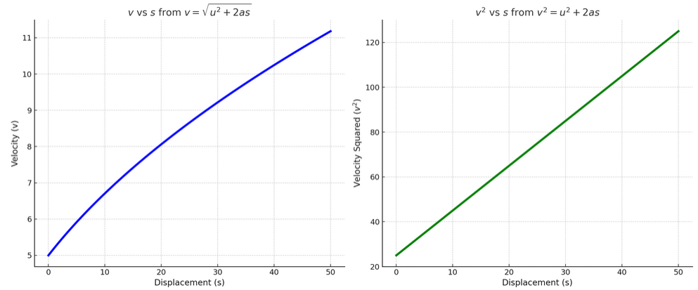
• Gradient = \( 2a \)
• y-intercept = \( u^2 \)
• Only valid for motion with constant acceleration.