Introduction to the Concept of a Limit
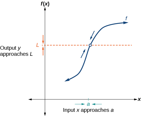
A limit describes the value that a function \( f(x) \) approaches as the input \( x \) gets closer to a particular point.
\( \lim_{x \to a} f(x) = L \)
This means that as \( x \) gets arbitrarily close to \( a \), \( f(x) \) gets arbitrarily close to \( L \).
Important points:
- The limit depends on the behavior of \( f(x) \) near \( x = a \), not necessarily at \( x = a \).
- The limit may exist even if \( f(a) \) is undefined.
- Limits can be found by direct substitution, simplification, or graphing.
Notation: Left-hand limit: \( \lim_{x \to a^-} f(x) \) Right-hand limit: \( \lim_{x \to a^+} f(x) \) If both are equal, the limit exists at \( a \).
Example:
Find the limit:
\( \lim_{x \to 2} \frac{x^2 – 4}{x – 2} \)
▶️ Answer/Explanation
Factor the numerator
\( \frac{(x – 2)(x + 2)}{x – 2} \)
Simplify
\( = x + 2 \), for \( x \neq 2 \)
Substitute \( x = 2 \)
\( = 2 + 2 = 4 \)
\( \lim_{x \to 2} \frac{x^2 – 4}{x – 2} = 4 \)
Estimating the Value of a Limit from a Table and Graph
When it is difficult or impossible to compute a limit algebraically, we can estimate it:
Using a table:
Calculate \( f(x) \) for values of \( x \) that approach \( a \) from both sides. If \( f(x) \) approaches the same number, that is the estimated limit.
Notation: If the table suggest the same value, we write:
\( \lim_{x \to a} f(x) = L \)
Example:
Estimate \( \lim_{x \to 1} \frac{x^2 – 1}{x – 1} \) using a table of values.
▶️ Answer/Explanation
Step 1: Make a table
| x | f(x) |
|---|---|
| 0.9 | 1.9 |
| 0.99 | 1.99 |
| 0.999 | 1.999 |
| 1.001 | 2.001 |
| 1.01 | 2.01 |
| 1.1 | 2.1 |
Step 2: Estimate from table
As \( x \to 1 \), \( f(x) \) approaches 2 from both sides.
Conclusion: \( \lim_{x \to 1} \frac{x^2 – 1}{x – 1} = 2 \) (estimated from the table and graph would confirm this)
Example:
The table below gives values of \( f(x) \) near \( x = 3 \). Estimate \( \lim_{x \to 3} f(x) \).
| x | f(x) |
|---|---|
| 2.9 | 7.9 |
| 2.99 | 7.99 |
| 2.999 | 7.999 |
| 3.001 | 8.001 |
| 3.01 | 8.01 |
| 3.1 | 8.1 |
▶️ Answer/Explanation
Looking at the table, as \( x \) approaches 3 from both sides:
- From the left: \( f(x) \) approaches values near 8 (7.9 → 7.99 → 7.999)
- From the right: \( f(x) \) approaches values near 8 (8.001 → 8.01 → 8.1)
Since \( f(x) \) approaches 8 from both sides:
\( \lim_{x \to 3} f(x) = 8 \)
Using a graph:
Observe the \( y \)-values of \( f(x) \) as \( x \) approaches \( a \). The height the curve approaches is the limit.
Notation: If the graph suggest the same value, we write:
\( \lim_{x \to a} f(x) = L \)
Example:
Using the graph of the function y=f(x) shown in Figure, estimate the following limits.
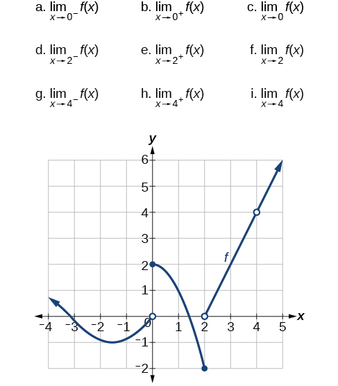
▶️ Answer/Explanation
Solution:
- a. 0
- b. 2;
- c. does not exist
- d.−2
- e. 0
- f. does not exist
- g. 4
- h. 4
- i. 4
Informal Understanding of the Gradient of a Curve as a Limit
The gradient of a curve at a point is the slope of the tangent line at that point. Since a curve doesn’t have a single gradient between two points, we estimate the gradient at a point by considering the gradient of a chord (secant) and letting the two points get infinitely close.
If we take two points on the curve \( (x, f(x)) \) and \( (x + h, f(x + h)) \), the gradient of the chord is:
\( \frac{f(x + h) – f(x)}{h} \)
As \( h \to 0 \), this approaches the gradient of the tangent:
\( \lim_{h \to 0} \frac{f(x + h) – f(x)}{h} \)
This limit gives the derivative at \( x \), which is the gradient of the curve at that point.
Example:
Estimate the gradient of \( f(x) = x^2 \) at \( x = 2 \) by computing the chord gradient for \( h = 0.1 \), \( 0.01 \), and \( 0.001 \).
▶️ Answer/Explanation
Gradient formula:
\( \frac{(2 + h)^2 – 2^2}{h} = \frac{(4 + 4h + h^2) – 4}{h} = \frac{4h + h^2}{h} = 4 + h \)
Calculate for each \( h \):
- \( h = 0.1 \): \( 4 + 0.1 = 4.1 \)
- \( h = 0.01 \): \( 4 + 0.01 = 4.01 \)
- \( h = 0.001 \): \( 4 + 0.001 = 4.001 \)
As \( h \to 0 \), the gradient approaches 4.
Conclusion: The gradient of the curve at \( x = 2 \) is 4.