The Graph of \( y = |f(x)| \)
The graph of \( y = |f(x)| \) can be obtained from the graph of \( y = f(x) \) by:
- Leaving the part of the graph where \( f(x) \ge 0 \) unchanged.
- Reflecting the part of the graph where \( f(x) < 0 \) in the x-axis (make negative y-values positive).
Example
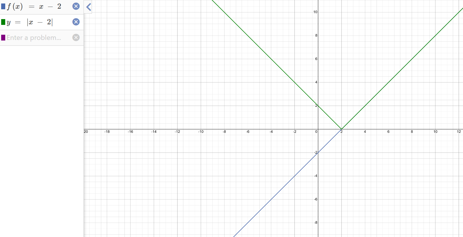
Given \( f(x) = x – 2 \), sketch \( y = |f(x)| \).
▶️ Answer/Explanation
- Plot \( y = x – 2 \). This is a straight line crossing the x-axis at \( x = 2 \).
- For \( x \ge 2 \): The graph stays the same.
- For \( x < 2 \): The negative y-values are reflected above the x-axis.
Use a graphing tool (Desmos, GeoGebra, GDC) to plot both \( y = x – 2 \) and \( y = |x – 2| \) to visualize the reflection.
The Graph of \( y = f(|x|) \)
The graph of \( y = f(|x|) \) can be obtained by:
- Keeping the part of the graph for \( x \ge 0 \) unchanged.
- Reflecting that part of the graph across the y-axis (mirror image).
Example
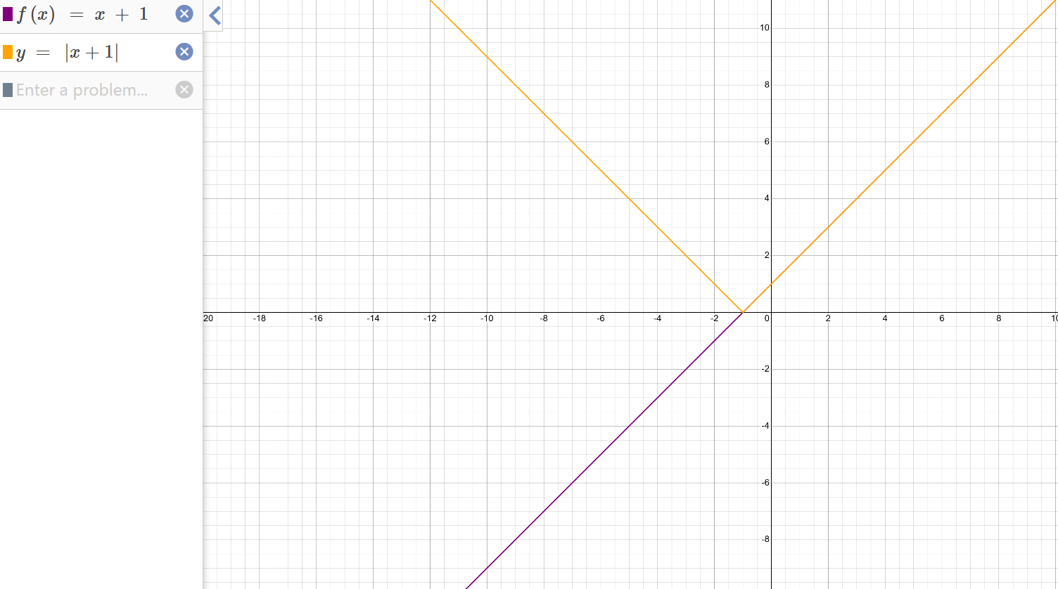
Given \( f(x) = x + 1 \), sketch \( y = f(|x|) \).
▶️ Answer/Explanation
- For \( x \ge 0 \): \( y = x + 1 \) (a straight line starting at (0,1)).
- For \( x < 0 \): The graph is the reflection of \( y = x + 1 \) for positive x, so it appears as \( y = (-x) + 1 \).
Use a graphing tool (Desmos, GeoGebra, GDC) to visualize both \( y = f(x) \) and \( y = f(|x|) \).
The Graph of \( y = \frac{1}{f(x)} \)
- The graph has vertical asymptotes where \( f(x) = 0 \) (since division by zero is undefined).
- The graph approaches zero where \( f(x) \) is large (positive or negative).
- Where \( f(x) \) is positive, \( y = \frac{1}{f(x)} \) is positive. Where \( f(x) \) is negative, \( y = \frac{1}{f(x)} \) is negative.
Example
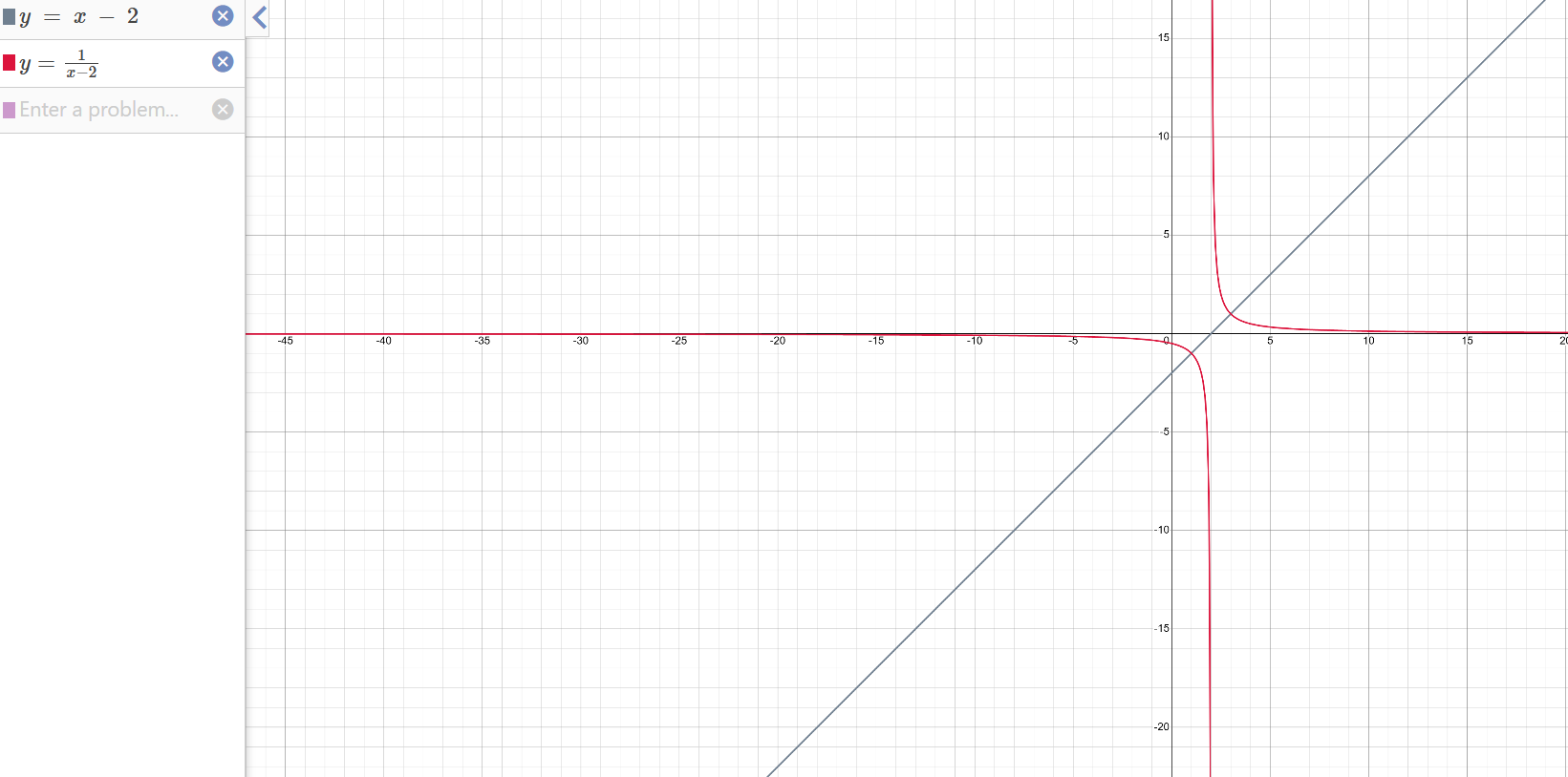
Given \( f(x) = x – 2 \), sketch \( y = \frac{1}{f(x)} \).
▶️ Answer/Explanation
- Since \( f(x) = 0 \) at \( x = 2 \), the graph of \( y = \frac{1}{f(x)} \) has a vertical asymptote at \( x = 2 \).
- For \( x > 2 \): \( f(x) > 0 \Rightarrow y = \frac{1}{f(x)} > 0 \).
- For \( x < 2 \): \( f(x) < 0 \Rightarrow y = \frac{1}{f(x)} < 0 \).
- As \( x \to \infty \), \( y \to 0^+ \). As \( x \to -\infty \), \( y \to 0^- \).
Graph both \( y = x – 2 \) and \( y = \frac{1}{x – 2} \) on Desmos or GDC to visualize their relationship.
The Graph of \( y = f(ax + b) \)
- The parameter \( a \) causes a horizontal stretch (if \( |a| < 1 \)) or compression (if \( |a| > 1 \)).
- The parameter \( b \) shifts the graph horizontally by \( -\frac{b}{a} \).
- If \( a < 0 \), there is also a reflection in the y-axis.
Example
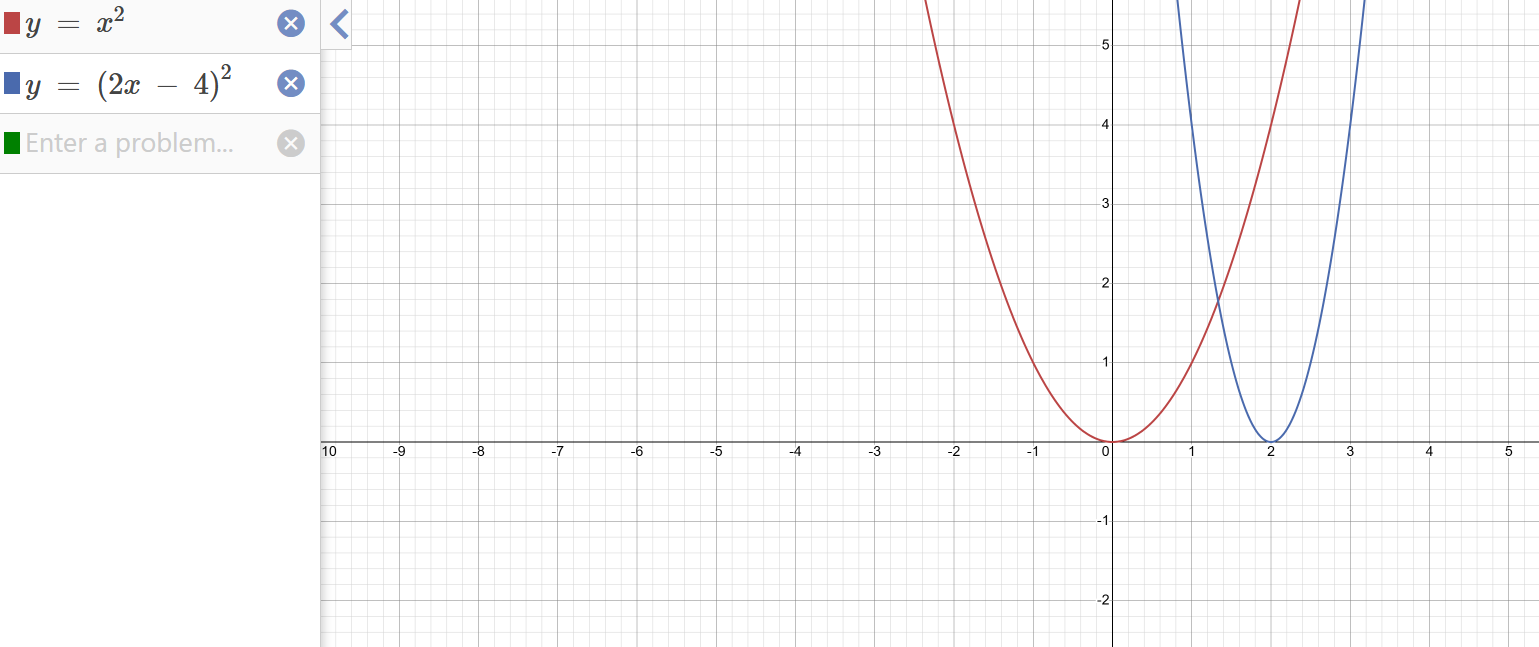
Given \( f(x) = x^2 \), sketch \( y = f(2x – 4) \).
▶️ Answer/Explanation
- The factor \( a = 2 \) causes a horizontal compression by factor \( \frac{1}{2} \).
- The term \( -4 \) causes a horizontal shift to the right by \( \frac{4}{2} = 2 \).
- The graph is a narrower parabola shifted right by 2 units.
Graph both \( y = x^2 \) and \( y = (2x – 4)^2 \) on Desmos or your GDC to compare.
The Graph of \( y = [f(x)]^2 \)
- The graph of \( y = [f(x)]^2 \) is always non-negative: \( y \ge 0 \).
- Where \( f(x) = 0 \), the graph of \( y = [f(x)]^2 \) also equals 0 (same x-intercepts as \( f(x) \)).
- Where \( f(x) \) is positive or negative, the output is positive (the graph lies above or on the x-axis).
- The shape becomes “flatter” at the x-axis near intercepts, and “steeper” where \( f(x) \) is large in magnitude.
Example
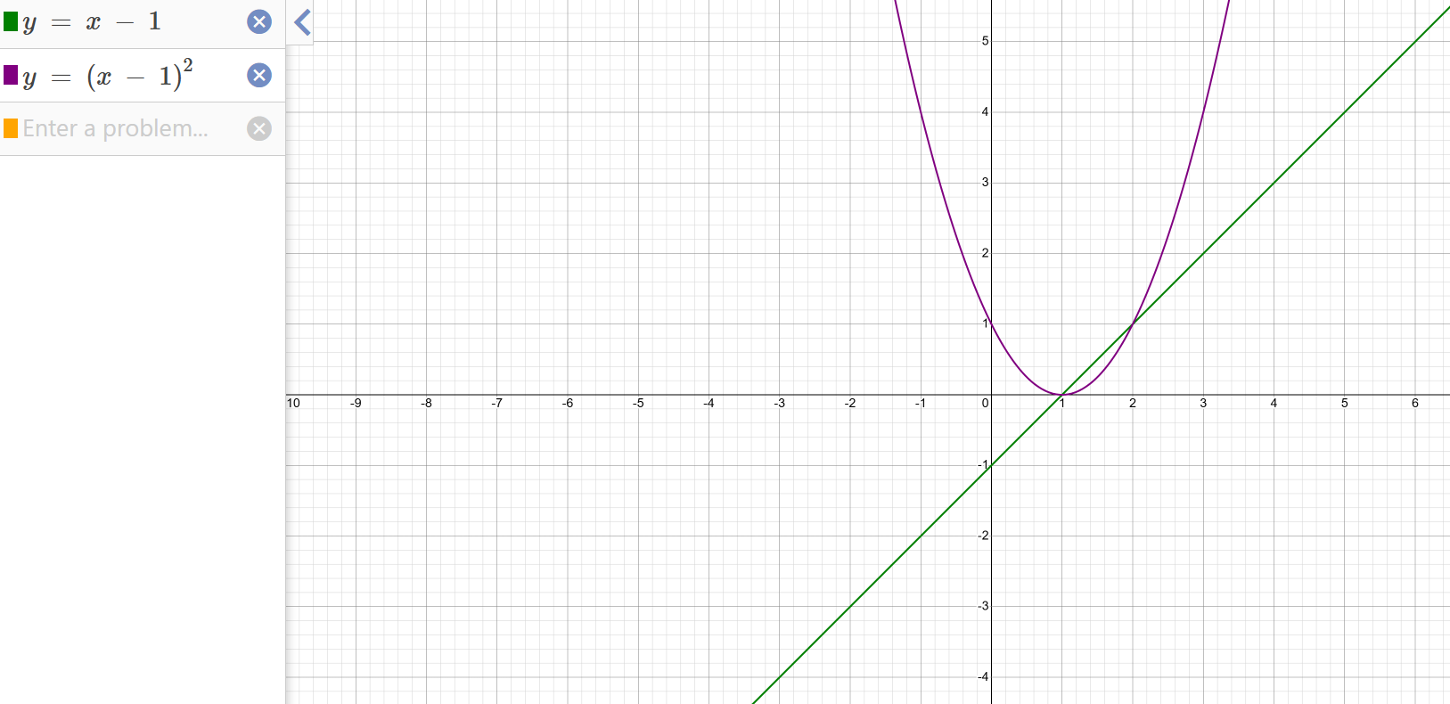
Given \( f(x) = x – 1 \), sketch \( y = [f(x)]^2 = (x – 1)^2 \).
▶️ Answer/Explanation
- The graph is \( y = (x – 1)^2 \), a parabola with vertex at \( (1, 0) \).
- It touches the x-axis at \( x = 1 \) (where \( f(x) = 0 \)).
- The entire graph lies above or on the x-axis, since squaring produces non-negative values.
Graph both \( y = x – 1 \) and \( y = (x – 1)^2 \) on Desmos or your GDC to see how squaring transforms the line into a parabola.
Solving Modulus Equations and Inequalities
Modulus (or absolute value) equations and inequalities involve expressions like \( |f(x)| \). These represent the distance of \( f(x) \) from zero, and are always non-negative.
General approach for solving \( |f(x)| > a \):
- If \( a > 0 \): Solve both
- \( f(x) > a \)
- \( f(x) < -a \)
- If \( a = 0 \): Solve
- \( f(x) \ne 0 \)
- If \( a < 0 \): The inequality is always true (because modulus is non-negative).
General approach for solving \( |f(x)| < a \):
- If \( a > 0 \): Solve
- \( -a < f(x) < a \)
- If \( a \le 0 \): No solution (modulus is always ≥ 0).
Steps when solving modulus equations or inequalities:
- Set up the two cases (positive and negative) as required by the inequality or equation.
- Solve each case algebraically or graphically.
- Consider the domain of \( f(x) \), especially for functions like \( \arccos(x) \), \( \ln(x) \), etc.
- Write the combined solution set.
- If needed, verify solutions using graphing technology (GDC, Desmos, GeoGebra).
Example
Solve the inequality:
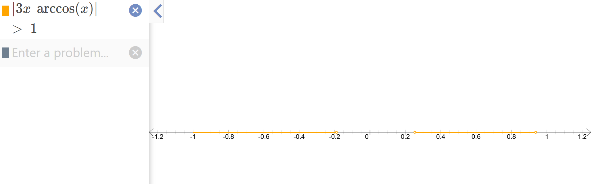
\( |3x \arccos(x)| > 1 \)
▶️ Answer/Explanation
The inequality means:
\( 3x \arccos(x) > 1 \) or \( 3x \arccos(x) < -1 \).
Since \( \arccos(x) \) is only defined for \( -1 \le x \le 1 \), restrict domain:
\( -1 \le x \le 1 \).
Graphically or with technology (Desmos / GDC), solve:
\( 3x \arccos(x) = 1 \)
\( 3x \arccos(x) = -1 \)
(Use GDC or software: e.g., solutions near \( x \approx 0.253 \) and \( x \approx -0.189\))
Write the solution set:
\( x \in (-1, -0.189) \cup (0.253, 1) \)
Use the graph of \( y = 3x \arccos(x) \) and \( y = 1 \), \( y = -1 \) to visualize intersections and solution regions.