Home / IB DP Maths 2026, 2027 & 2028 / IB Math Analysis and Approach HL / MAA HL Study Notes / Intersections of a line with a planes Study Notes

IB Mathematics AA Measures of central tendency Study Notes

IB Mathematics AA Measures of central tendency Study Notes

IB Mathematics AA Measures of central tendency Study Notes

IB Mathematics AA Measures of central tendency Notes Offer a clear explanation of Measures of central tendency, including various formula, rules, exam style questions as example to explain the topics. Worked Out examples and common problem types provided here will be sufficient to cover for topic Measures of central tendency.

Measures of Central Tendency

Measures of Central Tendency

Measures of central tendency describe a single value that represents the center or typical value of a dataset. The most common measures are:

  • Mean (average): The sum of all data values divided by the number of data values.
  • Median: The middle value in an ordered dataset. If there is an even number of values, the median is the average of the two middle values.
  • Mode: The value(s) that occur most frequently in the dataset. A dataset may have one mode, more than one mode (bimodal or multimodal), or no mode.

Formula for the mean:

\( \text{Mean} = \frac{\sum x_i}{n} \)

where \( x_i \) represents each data value and \( n \) is the number of data values.

Key points:

  • The mean is sensitive to extreme values (outliers).
  • The median is more resistant to outliers and skewed data.
  • The mode is useful for categorical data or to identify the most common value(s).

Example:

Measures of Central Tendency, Given the dataset: 5, 7, 7, 10, 12, 12, 12, 15, 18

▶️ Answer/Explanation

Mean (average):
\( \text{Mean} = \frac{5 + 7 + 7 + 10 + 12 + 12 + 12 + 15 + 18}{9} \)
\( = \frac{98}{9} \approx 10.89 \)

Median (middle value):
Since the data has 9 values, the median is the 5th value:
5, 7, 7, 10, 12, 12, 12, 15, 18
Median = 12

Mode (most frequent value):
The value that appears most often is 12.
Mode = 12

Estimation of Mean from Grouped Data

Estimation of Mean from Grouped Data

When data is presented in grouped form (class intervals with frequencies), the exact data values are not known. Therefore, we estimate the mean by assuming that all values in a class are located at the class midpoint.

Estimated mean =\( \frac{\sum (f \cdot x)}{\sum f} \)

where:

  • \( f \) = frequency of each class
  • \( x \) = class midpoint = \( \frac{\text{lower limit} + \text{upper limit}}{2} \)

 Steps:

  1. Identify class intervals and their frequencies.
  2. Calculate the midpoint \( x \) for each class.
  3. Compute \( f \cdot x \) for each class.
  4. Sum all \( f \cdot x \) values and divide by total frequency \( \sum f \).

 Key points:

  • This method gives an approximate mean.
  • It is more accurate if class intervals are small and data is evenly distributed within classes.

Example:

Estimation of Mean from Grouped Data , The table below shows the scores of students in a test:

Score RangeFrequency
0 – 103
10 – 205
20 – 307
30 – 405
▶️ Answer/Explanation
Score RangeFrequencyMidpoint (x)f · x
0 – 103515
10 – 2051575
20 – 30725175
30 – 40535175

Total frequency: \( 3 + 5 + 7 + 5 = 20 \)

Sum of \( f \cdot x \): \( 15 + 75 + 175 + 175 = 440 \)

Estimated mean:
\( = \frac{440}{20} = 22 \)

Modal Class (Grouped Data)

Modal Class (Grouped Data)

In grouped data with equal class intervals, the modal class is the class interval that has the highest frequency.

 Key Points:

  • The modal class gives an estimate of where the mode (most common value) lies in the data.
  • It applies only when the class intervals are of equal width.
  • We can refine the estimate of the mode within this class using formulas (e.g. using frequency densities or interpolation if necessary).

Example

Class IntervalFrequency
0 – 105
10 – 2012
20 – 3018
30 – 4010

In grouped data Determine, the modal class .

▶️ Answer/Explanation
Class IntervalFrequency
0 – 105
10 – 2012
20 – 3018
30 – 4010

 Modal Class: The class interval 20 – 30 is the modal class as it has the highest frequency (18).

Measures of Dispersion

Measures of Dispersion

Measures of dispersion describe how spread out the values of a dataset are. Three common measures are:

Interquartile Range (IQR): The difference between the third quartile (Q3) and the first quartile (Q1).

\( \text{IQR} = Q_3 – Q_1 \)

Variance: The mean of the squared deviations from the mean. For a sample:

\( s^2 = \frac{1}{n-1} \sum (x_i – \overline{x})^2 \)

For a population:

\( \sigma^2 = \frac{1}{n} \sum (x_i – \mu)^2 \)

Standard Deviation: The square root of the variance. It is in the same unit as the original data.

\( s = \sqrt{s^2} \) for a sample,
\( \sigma = \sqrt{\sigma^2} \) for a population

Note:

  • The IQR is resistant to outliers and shows the spread of the middle 50% of data.
  • The variance and standard deviation account for all values in the dataset and are sensitive to outliers.

Example

Consider the dataset: 2, 4, 4, 4, 5, 5, 7, 9

Find the interquartile range (IQR), variance, and standard deviation.

▶️ Answer/Explanation

IQR:
Q1 = 4 (median of lower half: 2, 4, 4, 4)
Q3 = 7 (median of upper half: 5, 5, 7, 9)
IQR = Q3 – Q1 = 7 – 4 = 3

Mean:
\( \overline{x} = \frac{2 + 4 + 4 + 4 + 5 + 5 + 7 + 9}{8} = \frac{40}{8} = 5 \)

Variance (sample):
\( s^2 = \frac{(2-5)^2 + (4-5)^2 + (4-5)^2 + (4-5)^2 + (5-5)^2 + (5-5)^2 + (7-5)^2 + (9-5)^2}{7} \)
\( = \frac{9 + 1 + 1 + 1 + 0 + 0 + 4 + 16}{7} \)
\( = \frac{32}{7} \approx 4.57 \)

Standard deviation:
\( s = \sqrt{4.57} \approx 2.14 \)

Example

Calculate the sample standard deviation and variance of the data using GDC.

Data: 4, 8, 6, 5, 3

▶️ Answer/Explanation
  1. Using Technology (TI-83/84 or GDC):
    • Press STAT1: Edit
    • Enter numbers into L1: 4, 8, 6, 5, 3
    • Press STATCALC1-Var StatsL1ENTER
    • Read the results:
      • Mean \( \overline{x} = 5.2 \)
      • Sample standard deviation \( Sx \approx 2.28 \)
      • Sample variance \( s^2 = (2.28)^2 \approx 5.19 \)
  2. Hand-check:
    \( s^2 = \frac{(4-5.2)^2 + (8-5.2)^2 + (6-5.2)^2 + (5-5.2)^2 + (3-5.2)^2}{4} \)
    \( = \frac{1.44 + 7.84 + 0.64 + 0.04 + 4.84}{4} \)
    \( = \frac{14.8}{4} = 3.7 \)
    \( s = \sqrt{3.7} \approx 1.92 \)

Effect of Constant Changes on Data

Effect of Constant Changes on Data

Adding or subtracting a constant:

    • The mean increases or decreases by that constant.
    • The standard deviation and variance stay the same, because the spread of the data is unchanged.

Multiplying all data values by a constant:

    • The mean is multiplied by that constant.
    • The standard deviation and variance are multiplied by the absolute value of the constant (standard deviation by the constant, variance by the constant squared).

Example

Consider the data set: 2, 4, 6

  1. Add 3 to each data item:
  2. Multiply each data item by 2:

Find New mean and standard deviation

▶️ Answer/Explanation

Original mean = \( \frac{2 + 4 + 6}{3} = 4 \)

Original standard deviation ≈ \( 2 \) (assume calculated via technology)

  1. Add 3 to each data item:
    New data: 5, 7, 9
    New mean = \( 4 + 3 = 7 \)
    New standard deviation = \( 2 \) (unchanged)
  2. Multiply each data item by 2:
    New data: 4, 8, 12
    New mean = \( 4 \times 2 = 8 \)
    New standard deviation = \( 2 \times 2 = 4 \)

Quartiles of Discrete Data

Quartiles of Discrete Data

Quartiles divide ordered data into four equal parts:

    • Q1 (Lower quartile): 25% of the data is below Q1.
    • Q2 (Median): 50% of the data is below Q2.
    • Q3 (Upper quartile): 75% of the data is below Q3.

Steps to calculate quartiles:

    1. Order the data from smallest to largest.
    2. Find Q2 (the median).
    3. Find Q1 as the median of the lower half (not including Q2 if odd number of data).
    4. Find Q3 as the median of the upper half (not including Q2 if odd number of data).

Example

Find the quartiles of the data set:

3, 7, 8, 5, 12, 14, 21, 13, 18

▶️Answer/Explanation
  1. Order the data:
    3, 5, 7, 8, 12, 13, 14, 18, 21
  2. Q2 (Median):
    The 5th value: 12
  3. Q1 (Median of lower half: 3, 5, 7, 8):
    Average of 5 and 7: \( \frac{5 + 7}{2} = 6 \)
  4. Q3 (Median of upper half: 13, 14, 18, 21):
    Average of 14 and 18: \( \frac{14 + 18}{2} = 16 \)

Quartiles: Q1 = 6, Q2 = 12, Q3 = 16

Example

Suppose 100 students took an exam with scores between 1 and 60. The grouped frequency table is:

Grouped Table

Determine the quartiles, draw a box plot, and identify any outliers.

▶️ Answer/Explanation

 Use cumulative frequency diagram.


  • \( Q_1 \): 25th percentile ≈ 25
  • \( Q_2 \): 50th percentile (Median) ≈ 38
  • \( Q_3 \): 75th percentile ≈ 46

Draw Box and Whisker Plot

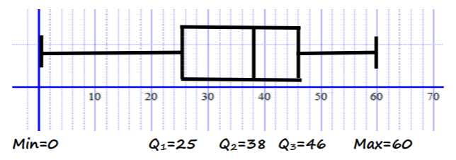
 Calculate IQR and check for outliers

$ \text{IQR} = Q_3 – Q_1 = 46 – 25 = 21 $

$ \text{Lower boundary} = Q_1 – 1.5 \times \text{IQR} = 25 – 1.5 \times 21 = -6.5 $

$ \text{Upper boundary} = Q_3 + 1.5 \times \text{IQR} = 46 + 1.5 \times 21 = 77.5 $

Conclusion: No outliers exist in the data set.

Scroll to Top