The Normal Distribution and Curve

The normal distribution is a continuous probability distribution that is symmetric about its mean. It describes many natural phenomena (e.g. heights, test scores) and is often used as an approximation for binomial distributions when \( n \) is large.

\( X \sim N(\mu, \sigma^2) \)

where:

• \( \mu \) = mean (center of the distribution)
• \( \sigma^2 \) = variance
• \( \sigma \) = standard deviation (measure of spread)

The probability density function is:

\( f(x) = \frac{1}{\sigma \sqrt{2\pi}} e^{ – \frac{(x – \mu)^2}{2 \sigma^2}} \)

Properties of the Normal Distribution

• It is bell-shaped and symmetric about \( \mu \).
• The mean, median, and mode are equal: \( \mu = \text{median} = \text{mode} \).
• Approximately 68% of values lie within \( \mu \pm \sigma \).
• Approximately 95% of values lie within \( \mu \pm 2\sigma \).
• Approximately 99.7% of values lie within \( \mu \pm 3\sigma \).
• The total area under the curve is 1 (represents total probability).

Diagrammatic Representation

A normal distribution curve is smooth and bell-shaped. The highest point is at \( x = \mu \). The curve approaches but never touches the horizontal axis (asymptotic).

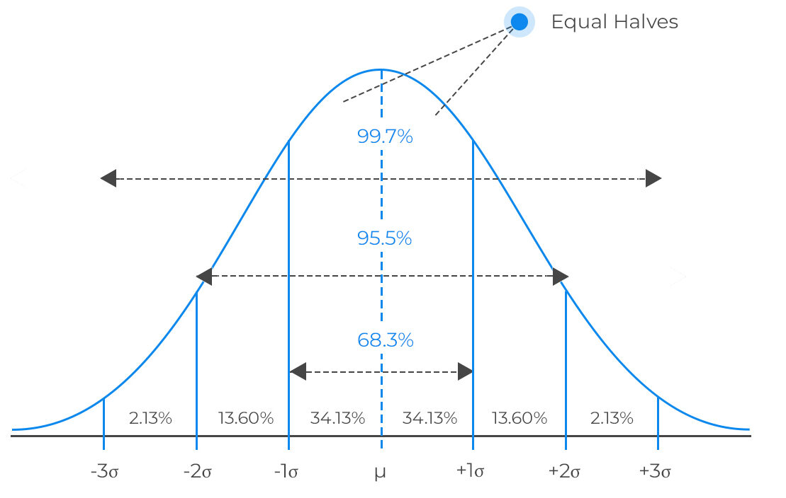
Diagram description:

• Horizontal axis labeled \( x \)
• Curve centered at \( \mu \)
• Vertical lines at \( \mu \), \( \mu \pm \sigma \), \( \mu \pm 2\sigma \), \( \mu \pm 3\sigma \)
• Shading for areas representing 68%, 95%, and 99.7%

Note: In practice, values of normal probabilities are found using technology (GDC, calculator) or standard normal tables.