Definite Integrals Using Technology
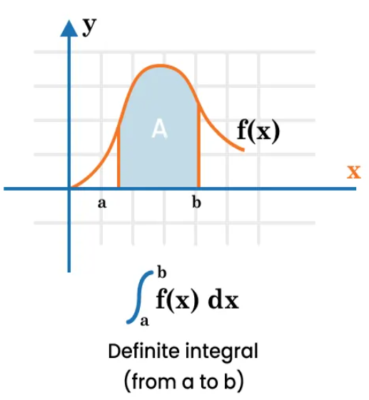
A definite integral calculates the area under the curve of \( f(x) \) between two bounds \( a \) and \( b \):
\( \int_a^b f(x)\, dx \)
How to compute using technology:
- Enter the function into the calculator or graphing tool.
- Access the integral or calculation menu.
- TI-Nspire: Menu → Calculus → Integral → enter bounds and function.
- Casio: Interactive → Calculate → ∫ → enter bounds and function.
- Desmos: Type
integrate(f(x), a, b)directly.
- The tool computes and displays the numerical value of the integral.
Technology will handle even complicated integrals where manual work would be slow or prone to error.
Example:
Use technology to compute: \( \int_1^3 \left( 2x^2 – x + 1 \right) dx \)
▶️ Answer/Explanation
- Enter: \( 2x^2 – x + 1 \) into the graphing calculator or Desmos.
- Choose integral calculation:
- TI-Nspire: Menu → Calculus → Integral → enter 1 as lower limit, 3 as upper limit → select function.
- Casio: Interactive → Calculate → ∫ → enter 1, 3, and function.
- Desmos: Type:
integrate(2x^2 - x + 1, 1, 3)
- The calculator shows: \( \int_1^3 (2x^2 – x + 1) dx = 14 \)
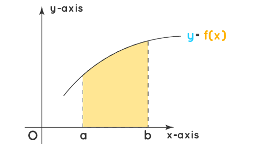
Area Under a Curve \( y = f(x) \) and the x-axis (where \( f(x) > 0 \))
If \( f(x) \ge 0 \) on an interval \([a, b]\), the area between the curve and the x-axis is:
\( \text{Area} = \int_a^b f(x) \, dx \)
The integral gives the exact area beneath the curve from \( x = a \) to \( x = b \).
When \( f(x) > 0 \), the integral directly gives the positive area.
How to compute:
- Identify the interval \([a, b]\).
- Set up and evaluate the definite integral: \( \int_a^b f(x) dx \)
- Use technology or manual integration.
Example:
Find the area enclosed by the curve \( y = x^2 + 1 \) and the x-axis from \( x = 0 \) to \( x = 2 \).
▶️ Answer/Explanation
\( \text{Area} = \int_0^2 (x^2 + 1) dx \)
Integrate
\( = \left[ \frac{x^3}{3} + x \right]_0^2 \)
Compute the result
\( = \left( \frac{8}{3} + 2 \right) – \left( 0 + 0 \right) = \frac{8}{3} + 2 = \frac{8}{3} + \frac{6}{3} = \frac{14}{3} \)
Final Answer:
The area is: \( \frac{14}{3} \text{ square units} \)
Using Technology to Understand Area Under a Curve
Dynamic geometry tools (such as GeoGebra) and graphing calculators (such as TI-Nspire, Casio GDC, or Desmos) are valuable in exploring and understanding the concept of area under a curve.
Example of using technology:
In Desmos, you can enter: integrate(f(x), a, b) and visually display the area by shading.
In TI-Nspire / Casio GDC: Menu → Calculus → Integral → select bounds → shaded region appears automatically.
Example:
Use graphing software to find the area under \( y = 2x + 1 \) from \( x = 1 \) to \( x = 4 \).
▶️ Answer/Explanation
- Enter \( f(x) = 2x + 1 \) into the graphing calculator or Desmos.
- Set integral bounds: \( x = 1 \) and \( x = 4 \).
- Use integral tool:
- TI-Nspire: Menu → Calculus → Integral → select bounds → shaded region appears + area displayed.
- Desmos: Type:
integrate(2x + 1, 1, 4).
- The technology displays: \( \int_1^4 (2x + 1) dx = 18 \)
Velocity-Time Graphs (with Technology)
A velocity-time graph represents how velocity \( v(t) \) of an object changes over time.
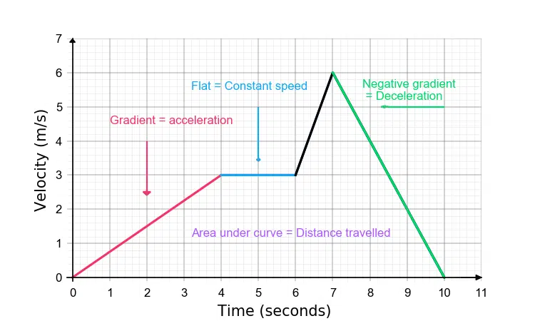
- The gradient of the graph: gives the acceleration \( a(t) \).
- The area under the graph (between the curve and the time axis): gives the displacement or distance travelled.
Dynamic geometry and graphing software (TI-Nspire, Casio fx-CG50, Desmos, GeoGebra) help:
- Visualize how velocity changes over time
- Automatically compute gradients (acceleration) at points
- Compute areas under curves (displacement)
- Animate motion to link graph to physical movement
Technology Workflow:
- Enter \( v(t) \) into graphing tool.
- Plot the velocity-time graph.
- Use slope/derivative tools to find acceleration at specific times.
- Use integral tools to compute displacement over intervals.
Example:
A particle moves with velocity \( v(t) = t^2 – 2t + 3 \) m/s. Use technology to:
- Find its displacement from \( t = 0 \) to \( t = 3 \) seconds.
- Find its acceleration at \( t = 2 \) seconds.
▶️ Answer/Explanation
- Enter \( v(t) = t^2 – 2t + 3 \) into the GDC or Desmos.
- Plot graph for \( 0 \le t \le 3 \).
- Use integral tool:
TI-Nspire: Menu → Calculus → Integral → lower: 0, upper: 3 → function: \( v(t) \)
Casio: Interactive → Calculate → ∫ → enter 0, 3, \( v(t) \)
Desmos:integrate(t^2 - 2t + 3, 0, 3) - The calculator shows: \( \int_0^3 (t^2 – 2t + 3) dt = 7.5 \text{ m} \)
- Use derivative tool at \( t = 2 \):
TI-Nspire: Menu → Analyze Graph → Derivative → point: 2
Casio: Interactive → Calculate → d/dt → enter 2
Or compute manually: \( a(t) = v'(t) = 2t – 2 \) \( a(2) = 2(2) – 2 = 2 \text{ m/s}^2 \)