Home / IB DP Maths 2026, 2027 & 2028 / IB Math Analysis and Approach HL / MAA HL Study Notes / Intersections of a line with a planes Study Notes

IB Mathematics AA Standardization of normal variables Study Notes

IB Mathematics AA Standardization of normal variables Study Notes

IB Mathematics AA Standardization of normal variables Study Notes

IB Mathematics AA Standardization of normal variables Notes Offer a clear explanation of Standardization of normal variables, its mean and variance, including various formula, rules, exam style questions as example to explain the topics. Worked Out examples and common problem types provided here will be sufficient to cover for topic Standardization of normal variables, its mean and variance.

Standardization of Normal Variables (z-values)

Standardization of Normal Variables (z-values)

Standardization is the process of converting a normal variable \( X \) into a standard normal variable \( Z \), which has mean 0 and standard deviation 1.

The formula for the standardized value is:

\( z = \frac{x – \mu}{\sigma} \)

Where:

  • \( x \) = value of the variable
  • \( \mu \) = mean of the distribution
  • \( \sigma \) = standard deviation of the distribution

The standardized value \( z \) tells you how many standard deviations \( x \) is above or below the mean.

Interpretation:

  • \( z = 0 \): \( x \) is at the mean
  • \( z > 0 \): \( x \) is above the mean
  • \( z < 0 \): \( x \) is below the mean

Example:

The heights of adult males are normally distributed with a mean of 175 cm and a standard deviation of 8 cm. Find the standardized \( z \)-value for a man who is 190 cm tall. Interpret the result.

▶️ Answer/Explanation

\( x = 190 \), \( \mu = 175 \), \( \sigma = 8 \)

standardization formula

\( z = \frac{190 – 175}{8} = \frac{15}{8} = 1.875 \)

Interpretation:

The man is 1.875 standard deviations taller than the mean height.

Example:

The weight of apples in a supermarket is normally distributed with mean \( 150 \) g and standard deviation \( 15 \) g.

(a) Find the probability that a randomly chosen apple weighs less than 130 g.
(b) Find the weight that marks the top 10% of heaviest apples.

▶️ Answer/Explanation

(a) Probability that apple weighs less than 130 g

Standardize: \( z = \frac{130 – 150}{15} = \frac{-20}{15} = -1.33 \)

Using GDC: normalcdf(-1E99, 130, 150, 15)
or directly: normalcdf(-1E99, -1.33, 0, 1) if using z

Result: \( P(X < 130) \approx 0.0918 \)

(b) Find weight for top 10% (90th percentile)

Use inverse normal:

GDC: invNorm(0.90, 150, 15)

Result: \( x \approx 169.2 \) g

Inverse Normal Calculations (Unknown Mean and Standard Deviation)

Inverse Normal Calculations (Unknown Mean and Standard Deviation)

In some problems, you are given a probability and a value of the variable, and you are asked to find the mean \( \mu \) and/or standard deviation \( \sigma \) of the normal distribution.

Key idea: Standardize and set up an equation involving z-values:

\( z = \frac{x – \mu}{\sigma} \)

You use technology (GDC or tables) to find the z-value corresponding to the given probability.

Example:

A machine fills cereal packets. The masses are normally distributed.
It is known that 5% of packets weigh less than 490 g, and 10% weigh more than 510 g.
Find the mean and standard deviation of the mass.

▶️ Answer/Explanation

Express probabilities in terms of z

\( P(X < 490) = 0.05 \Rightarrow z_1 = \text{invNorm}(0.05) \approx -1.645 \)
\( P(X > 510) = 0.10 \Rightarrow P(X < 510) = 0.90 \Rightarrow z_2 = \text{invNorm}(0.90) \approx 1.281 \)

Set up equations

\( \frac{490 – \mu}{\sigma} = -1.645 \quad \Rightarrow 490 – \mu = -1.645 \sigma \)
\( \frac{510 – \mu}{\sigma} = 1.281 \quad \Rightarrow 510 – \mu = 1.281 \sigma \)

Solve the system

Subtract the two equations:
\( (510 – \mu) – (490 – \mu) = 1.281 \sigma + 1.645 \sigma \)
\( 20 = 2.926 \sigma \Rightarrow \sigma = 20 / 2.926 \approx 6.84 \)

Use \( \sigma \) to find \( \mu \):
\( 490 – \mu = -1.645 \times 6.84 \Rightarrow 490 – \mu = -11.25 \Rightarrow \mu = 501.25 \)

Final answer:

Mean \( \mu \approx 501.25 \) g, Standard deviation \( \sigma \approx 6.84 \) g

Example:

In a standardized test, scores are normally distributed.
You are told that 20% of students score below 60, and 10% score above 85.
Find the mean and standard deviation of the test scores.

▶️ Answer/Explanation

Translate probabilities into z-values

For \( P(X < 60) = 0.20 \):
Use GDC: invNorm(0.20) → \( z_1 \approx -0.8416 \)

For \( P(X > 85) = 0.10 \Rightarrow P(X < 85) = 0.90 \):
Use GDC: invNorm(0.90) → \( z_2 \approx 1.2816 \)

Set up equations using z formula

\( \frac{60 – \mu}{\sigma} = -0.8416 \Rightarrow 60 – \mu = -0.8416 \sigma \)
\( \frac{85 – \mu}{\sigma} = 1.2816 \Rightarrow 85 – \mu = 1.2816 \sigma \)

Subtract:
\( 85 – 60 = 1.2816 \sigma + 0.8416 \sigma \)
\( 25 = 2.1232 \sigma \Rightarrow \sigma = 25 / 2.1232 \approx 11.78 \)

\( 60 – \mu = -0.8416 \times 11.78 \Rightarrow 60 – \mu = -9.91 \Rightarrow \mu = 60 + 9.91 = 69.91 \)

Final result:

Mean \( \mu \approx 69.9 \), standard deviation \( \sigma \approx 11.8 \)

Z Score Table

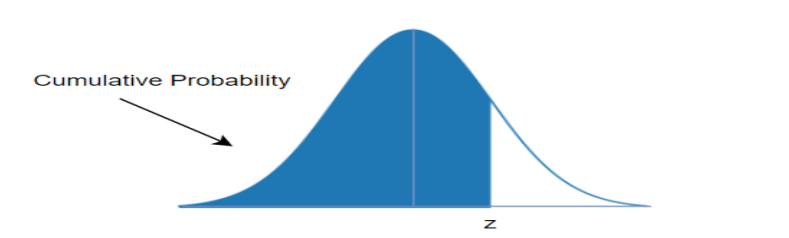
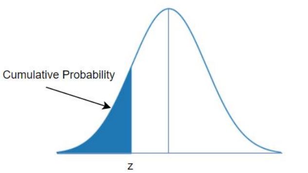
Z score table also called as standard normal table is used to determine corresponding area or probability to z score value.

1. Positive Z Score Table or Chart

Z \ ΔZ0.000.010.020.030.040.050.060.070.080.09
0.00.50000.50400.50800.51200.51600.51990.52390.52790.53190.5359
0.10.53980.54380.54780.55170.55570.55960.56360.56750.57140.5753
0.20.57930.58320.58710.59100.59480.59870.60260.60640.61030.6141
0.30.61790.62170.62550.62930.63310.63680.64060.64430.64800.6517
0.40.65540.65910.66280.66640.67000.67360.67720.68080.68440.6879
0.50.69150.69500.69850.70190.70540.70880.71230.71570.71900.7224
0.60.72570.72910.73240.73570.73890.74220.74540.74860.75170.7549
0.70.75800.76110.76420.76730.77040.77340.77640.77940.78230.7852
0.80.78810.79100.79390.79670.79950.80230.80510.80780.81060.8133
0.90.81590.81860.82120.82380.82640.82890.83150.83400.83650.8389
1.00.84130.84380.84610.84850.85080.85310.85540.85770.85990.8621
1.10.86430.86650.86860.87080.87290.87490.87700.87900.88100.8830
1.20.88490.88690.88880.89070.89250.89440.89620.89800.89970.9015

2. Negative Z Score Table or Chart

Z \ ΔZ0.000.010.020.030.040.050.060.070.080.09
-0.10.46020.45620.45220.44830.44430.44040.43640.43250.42860.4247
-0.20.42070.41680.41290.40900.40520.40130.39740.39360.38970.3859
-0.30.38210.37830.37450.37070.36690.36320.35940.35570.35200.3483
-0.40.34460.34090.33720.33360.33000.32640.32280.31920.31560.3121
-0.50.30850.30500.30150.29810.29460.29120.28770.28430.28100.2776
-0.60.27430.27090.26760.26430.26110.25780.25460.25140.24830.2451
-0.70.24200.23890.23580.23270.22960.22660.22360.22060.21770.2148
-0.80.21190.20900.20610.20330.20050.19770.19490.19220.18940.1867
-0.90.18410.18140.17880.17620.17360.17110.16850.16600.16350.1611
-1.00.15870.15620.15390.15150.14920.14690.14460.14230.14010.1379
-1.10.13570.13350.13140.12920.12710.12510.12300.12100.11900.1170
-1.20.11510.11310.11120.10930.10750.10560.10380.10200.10030.0985
-1.30.09680.09510.09340.09180.09010.08850.08690.08530.08380.0823
-1.40.08080.07930.07780.07640.07490.07350.07210.07080.06940.0681

For Complete Table : Link

Scroll to Top