Adjacency Matrices
An adjacency matrix, also known as a connection matrix, is used to represent a simple labeled graph. It is a matrix where both the rows and columns correspond to the graph’s vertices. Each entry $(v_i, v_j)$ in the matrix is either 1 or 0, depending on whether the vertex $v_i$ is connected to $v_j$. If the graph does not contain self-loops, then the diagonal entries must all be 0. In the case of an undirected graph, the matrix is symmetric.

Example For the given the graph G , draw adjacency matrix(M).
▶️Answer/ExplanationSolution: 1s show a connection by an edge.
The matrix:
is called adjacency matrix(M). Notice that:
|


THE POWERS OF AN ADJACENCY MATRIX
For the adjacent matrix M of the graph:
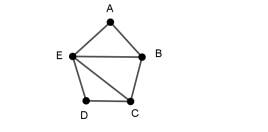
$M^2=\left(\begin{array}{lllll}2 & 1 & 2 & 1 & 1 \\ 1 & 3 & 1 & 2 & 2 \\ 2 & 1 & 3 & 1 & 2 \\ 1 & 2 & 1 & 2 & 1 \\ 1 & 2 & 2 & 1 & 4\end{array}\right)$
This matrix shows the number of walks of length 2.
For example:
there are 2 walks from A to A: ABA and AEA
there is only 1 walk from A to B: AEB (Note: Source incorrectly states AB which is length 1.)
there are 3 walks from B to B: BAB, BEB and BCB.
the main diagonal contains the degrees of the vertices (why? A walk of length 2 back to the start vertex must go out along an edge and back along the same edge, so the number of such walks equals the number of edges connected to the vertex, i.e., its degree.)
Similarly, $M^3$ shows the numbers of walks of length 3,
$M^3=\left(\begin{array}{lllll}2 & 5 & 3 & 3 & 6 \\ 5 & 4 & 7& 3 & 7 \\ 3 & 7 & 4 & 5 & 7 \\ 3 & 3 & 5 & 2 & 6 \\ 6 & 7 & 7 & 6 & 6\end{array}\right)$
Finally, look at the following sums:
$M+M^{2}$ shows the numbers of walks of length at most 2.
$M+M^{2}+M^{3}$ shows the numbers of walks of length at most 3.
Walks in Graphs and k-length Walks
Definition
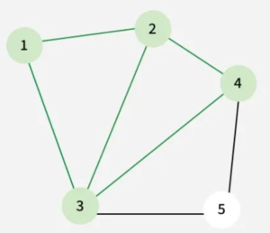
In graph theory, a walk is a sequence of vertices where each consecutive pair is connected by an edge. A walk of length \( k \) consists of exactly \( k \) edges. Walks can revisit vertices and edges.
In Above Figure, 1-> 2-> 3-> 4-> 2-> 1-> 3 is a walk.
Note: Walk can be open or closed.
Adjacency Matrix
The adjacency matrix \( A \) of a graph with \( n \) vertices is an \( n \times n \) matrix where:
- \( A_{ij} = 1 \) if there is an edge from vertex \( i \) to vertex \( j \)
- \( A_{ij} = 0 \) if there is no such edge
Walks and Powers of the Adjacency Matrix
The number of walks of length \( k \) from vertex \( i \) to vertex \( j \) is given by the \((i, j)\) entry of the matrix \( A^k \), the \( k^{\text{th}} \) power of the adjacency matrix.
Example: Consider the graph with the following adjacency matrix \( A \): $ A = \begin{bmatrix} 0 & 1 & 1 \\ 1 & 0 & 1 \\ 1 & 1 & 0 \end{bmatrix} $ Task: Find the number of walks of length 2 from vertex 1 to vertex 2. ▶️ Answer/ExplanationStep 1: Compute \( A^2 \) $A^2 = A \cdot A = \begin{bmatrix} 0 & 1 & 1 \\ 1 & 0 & 1 \\ 1 & 1 & 0 \end{bmatrix} \cdot \begin{bmatrix} 0 & 1 & 1 \\ 1 & 0 & 1 \\ 1 & 1 & 0 \end{bmatrix} = \begin{bmatrix} 2 & 1 & 1 \\ 1 & 2 & 1 \\ 1 & 1 & 2 \end{bmatrix}$ Step 2: Interpret the Result The entry \( (1, 2) \) in \( A^2 \) is \( 1 \). Conclusion: There is 1 walk of length 2 from vertex 1 to vertex 2. |
Weighted adjacency tables.
In a weighted graph, each edge has an associated numerical value called its weight. This weight often represents a quantity like distance, cost, or capacity associated with the connection between the vertices. For example, a map showing cities (vertices) and driving distances (weights) between them can be represented as a weighted graph.
Sometimes the edge alone is not enough to represent the information we want. For example, we want to include the distances between 5 cities:

The path ABCD has
$\text{Length = 3 [as it contains 3 edges]}$
$\text{Total weight = 27 [sum of weights 8+9+10=27]}$
We can represent the weighted graph by a weighted adjacency table.(we do not say matrix!).

Example: Consider a weighted graph with vertices A, B, C, and D, and the following edge weights:
Give Weighted Adjacency Table and explain that also. ▶️ Answer/ExplanationSolution: $\begin{array}{c|cccc} & A & B & C & D \\ \hline A & 0 & 3 & 5 & 4 \\ B & 3 & 0 & 0 & 7 \\ C & 5 & 0 & 0 & 2 \\ D & 4 & 7 & 2 & 0 \\ \end{array} $ This table assumes the graph is undirected, so it is symmetric. |
Transition systems were created by Andrei Markov, a Russian mathematician during the 19th century. A transition system can be used to represent the manner in which states change from one state to the next. For example a transition system can be used to represent the chance of rain or a dry day, given yesterday’s weather.
Consider the following statement for Traralgon’s weather in spring: “Long run data suggests that there is a 70% change that if today is dry, then tomorrow will also be dry. Also, if today is wet, there is an 80% chance that tomorrow will also be wet.”

The transition matrix (T) for the above example would be:

Example In Melbourne there are two major daily newspapers, The Age and the Herald Sun. Readers are fairly Construct a transition table ▶️Answer/ExplanationSolution: Transition table
Transition diagram
Transition matrix (T)
|


Page rank
Google’s success is based on an algorithm to rank webpages, the Page rank, named after Google founder Larry Page.
The basic idea is to determine how likely it is that a web user randomly gets to a given webpage. The webpages are then ranked by these probabilities.
Example Suppose the internet consisted of only the four webpages A,B, C,D linked as in the following graph:
▶️Answer/ExplanationSolution: Imagine a surfer following these links at random. For the probability $\text{PR}_n(A)$ that she is at $A$ (after $n$ steps), we add: the probability that she was at $B$ (at exactly one time step before), and left for $A$, the probability that she was at $C$, and left for $A$, the probability that she was at $D$, and left for $A$, Hence: $\text{PR}_n(A) = \text{PR}_{n-1}(B) \cdot \frac{1}{2} + \text{PR}_{n-1}(C) \cdot \frac{1}{1} + \text{PR}_{n-1}(D) \cdot \frac{0}{1}$ We can express this as a Markov matrix: $ The PageRank vector $\begin{bmatrix} \text{PR}(A) \\ \text{PR}(B) \\ \text{PR}(C) \\ \text{PR}(D) \end{bmatrix}$ is the long-term equilibrium. It is an eigenvector of the Markov matrix with eigenvalue 1. To find this vector, solve: $ Perform row reduction on: $ $ The PageRank vector is: $ Final Ranking: The corresponding ranking of the webpages is: $ |

Connection to Markov Chains
The concepts of adjacency matrices and transition matrices in graph theory have a strong connection to the study of Markov chains in probability theory.
Essentially, a Markov chain can be visually and mathematically represented as a weighted directed graph. In this representation:
- Vertices correspond to the different states of the Markov chain.
- Edges illustrate the possible transitions between these states.
- Edge weights represent the transition probabilities – the likelihood of moving from one state to another along a specific edge.
This graphical representation provides an intuitive way to understand the dynamics and transitions within a Markov chain.