Phase Portraits in Coupled Differential Equations
A phase portrait is a graphical representation that shows the trajectories of a dynamical system in the phase plane, illustrating how the system evolves over time from different initial conditions.
Consider the system of coupled first-order differential equations:
\(\frac{dx}{dt} = ax + by\)
\(\frac{dy}{dt} = cx + dy\)
Here, \(a\), \(b\), \(c\), and \(d\) are constants, and the system describes the rate of change of two variables \(x\) and \(y\) with respect to time \(t\).
Phase portraits help visualize the behavior of solutions for all initial points \((x_0, y_0)\) by plotting trajectories (paths) followed by the system in the plane.
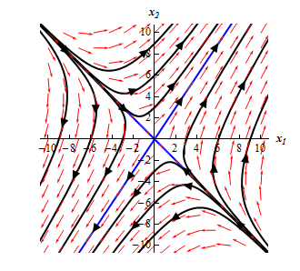
Example Sketch some trajectories for the system: \[ \begin{aligned} x_1′ &= x_1 + 2x_2 \\ x_2′ &= 3x_1 + 2x_2 \end{aligned} \quad \Rightarrow \quad \vec{x}’ = \begin{pmatrix} 1 & 2 \\ 3 & 2 \end{pmatrix} \vec{x} \] ▶️ Answer/ExplanationWe choose some points in the phase plane and compute the direction vectors by multiplying with the system matrix: \[ \vec{x} = \begin{pmatrix} -1 \\ 1 \end{pmatrix} \Rightarrow \vec{x}’ = \begin{pmatrix} 1 & 2 \\ 3 & 2 \end{pmatrix} \begin{pmatrix} -1 \\ 1 \end{pmatrix} = \begin{pmatrix} 1 \\ -1 \end{pmatrix} \] \[ \vec{x} = \begin{pmatrix} 2 \\ 0 \end{pmatrix} \Rightarrow \vec{x}’ = \begin{pmatrix} 1 & 2 \\ 3 & 2 \end{pmatrix} \begin{pmatrix} 2 \\ 0 \end{pmatrix} = \begin{pmatrix} 2 \\ 6 \end{pmatrix} \] \[ \vec{x} = \begin{pmatrix} -3 \\ -2 \end{pmatrix} \Rightarrow \vec{x}’ = \begin{pmatrix} 1 & 2 \\ 3 & 2 \end{pmatrix} \begin{pmatrix} -3 \\ -2 \end{pmatrix} = \begin{pmatrix} -7 \\ -13 \end{pmatrix} \] Interpretation:
This helps sketch the flow of solutions (trajectories) in the phase portrait. |
Key Features of Phase Portraits
Phase portraits consist of trajectories, also called orbits, representing solutions to the system for different initial conditions.
- Equilibrium points: Points where \(\frac{dx}{dt} = 0\) and \(\frac{dy}{dt} = 0\). The system remains at rest here.
- Stability: Determines whether trajectories move towards or away from equilibrium points.
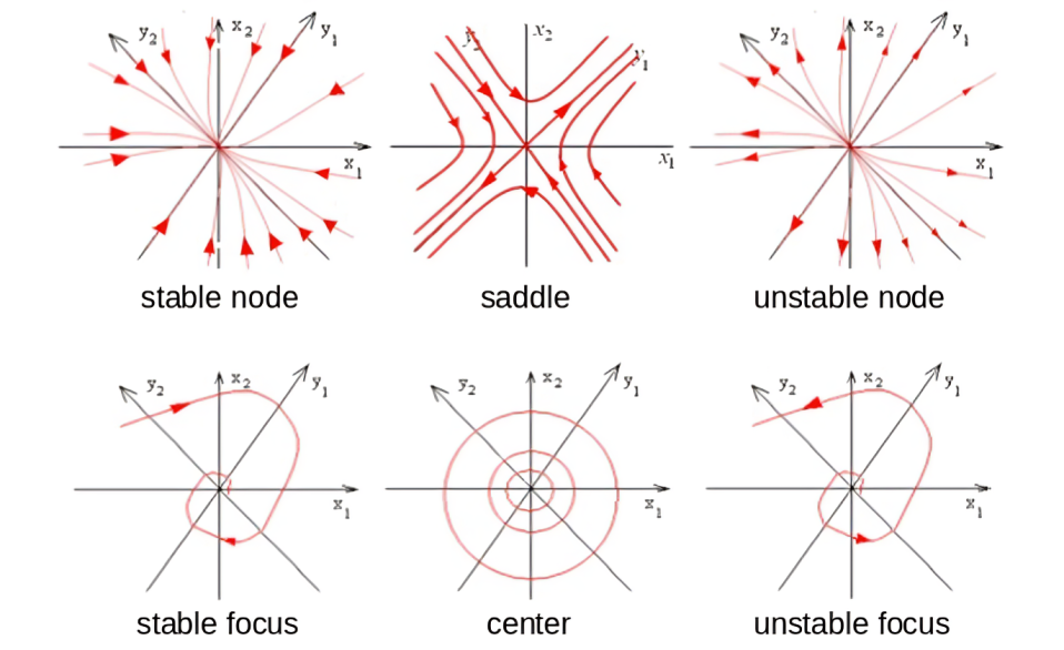
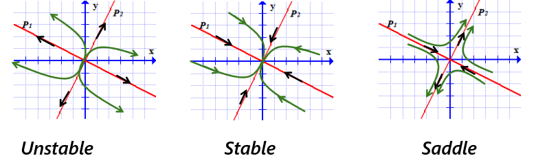
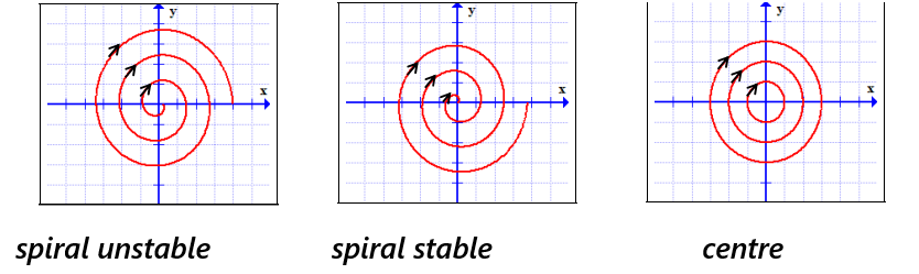
- Types of equilibrium points: Nodes, saddles, spirals, centers, depending on system parameters.
- Direction fields: Vector fields showing instantaneous direction of movement at any point.

Applications of Phase Portrait Analysis
Phase portraits are used widely in physics, biology, economics, and engineering to study systems such as:
- Mechanical oscillators (e.g., pendulums, springs)
- Electrical circuits (e.g., RLC circuits)
- Population dynamics (predator-prey models)
- Control systems stability
- Neural networks and biological rhythms
They provide visual insights into system stability, oscillations, and possible bifurcations.
Eigenvalues and Their Impact on Solutions
To analyze the system, we write it in matrix form:
\(\frac{d}{dt} \begin{bmatrix} x \\ y \end{bmatrix} = \begin{bmatrix} a & b \\ c & d \end{bmatrix} \begin{bmatrix} x \\ y \end{bmatrix}\)
The eigenvalues \(\lambda_1, \lambda_2\) of the coefficient matrix determine the nature of the equilibrium point at the origin:
Real and distinct eigenvalues
•If both $\lambda_1, \lambda_2 > 0$: unstable node
•If both $\lambda_1, \lambda_2 < 0$: stable node
•If $\lambda_1 < 0 < \lambda_2$: saddle point (unstable)
Real and repeated eigenvalues
• If there are enough linearly independent eigenvectors, we get a star node.
• If not, the system is an improper node (trajectories curve into/out of the same direction).
• Stability is determined by the sign of the repeated eigenvalue.
Complex eigenvalues $\lambda = a \pm bi$
Trajectories are spirals or centers.
• If $a > 0$: spiral out (unstable focus)
• If $a < 0$: spiral in (stable focus)
• If $a = 0$: center (neutral stability)
Zero eigenvalues
• Suggests a line of equilibrium points or degenerate behavior.
• System may not be asymptotically stable even if other eigenvalues are negative.
• Requires deeper qualitative or nonlinear analysis.
Example Find the eigenvalues of $ A = \begin{bmatrix} 3 & 4 \\ 2 & 1 \end{bmatrix} $ and interpret what they imply about the system behavior. ▶️ Answer/ExplanationSolve the characteristic equation: |
Sketching Trajectories
Trajectories are curves in the phase plane that represent solution paths. To sketch these:
- Find equilibrium points by solving \(ax + by = 0\) and \(cx + dy = 0\).
- Calculate eigenvalues and eigenvectors of the matrix \(\begin{bmatrix}a & b \\ c & d\end{bmatrix}\).
- Plot eigenvectors through the equilibrium point; these form the directions of trajectories.
- Determine behavior near equilibrium using eigenvalues’ sign and type.
- Draw curves moving along or spiraling around eigenvectors accordingly.
Exact Solutions for Real Distinct Eigenvalues
When eigenvalues \(\lambda_1 \neq \lambda_2\) are real and distinct, the general solution is:
$\begin{bmatrix} x \\ y \end{bmatrix} = C_1 \mathbf{v}_1 e^{\lambda_1 t} + C_2 \mathbf{v}_2 e^{\lambda_2 t} $
where \(\mathbf{v}_1, \mathbf{v}_2\) are eigenvectors associated with \(\lambda_1, \lambda_2\) and \(C_1, C_2\) are constants determined by initial conditions.
These solutions trace out trajectories in the phase plane shaped by the exponential growth/decay along eigenvectors.
Example Given eigenvalues \(\lambda_1=5\), \(\lambda_2=-1\) with eigenvectors $ \mathbf{v}_1 = \begin{bmatrix} 2 \\ 1 \end{bmatrix}, \quad \mathbf{v}_2 = \begin{bmatrix} 1 \\ -1 \end{bmatrix} $ Write the general solution of the system. ▶️ Answer/ExplanationThe general solution is: |