Euler Method
Concept:
Euler’s method is a numerical approach to approximate solutions of first order differential equations of the form:
$\frac{dy}{dx} = f(x, y), \quad y(x_0) = y_0$
Idea: Starting from the initial point \((x_0, y_0)\), we compute successive values using:
$ y_{n+1} = y_n + h f(x_n, y_n) $
where \( h \) is the step size and \( x_{n+1} = x_n + h \).
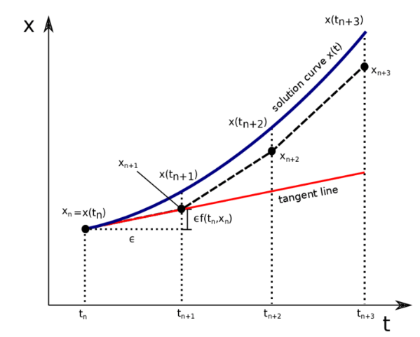
Euler’s method The dashed line shows the solution computed by successive iterations of Euler’s method. It diverges from the actual solution as errors accumulate over time.
GDC Tip: Use the Recursion feature:
Define \( X_0 = x_0 \), \( Y_0 = y_0 \) – \( X_{n+1} = X_n + h \) – \( Y_{n+1} = Y_n + h \cdot f(X_n, Y_n) \)
Example Use Euler’s method with \( h = 0.1 \) to approximate \( y(0.1) \) for \( \frac{dy}{dx} = x + y \), with \( y(0) = 1 \) ▶️Answer/ExplanationStep: $ y_1 = y_0 + h(x_0 + y_0) = 1 + 0.1(0 + 1) = 1.1$ |
Using Spreadsheets for Euler’s Method
Euler’s Method provides a numerical technique to approximate solutions to first-order differential equations of the form:
\(\frac{dy}{dx} = f(x, y), \quad y(x_0) = y_0\)
A spreadsheet (e.g. Excel or Google Sheets) allows for iterative computation through columns for:
- x values (e.g., \(x_0, x_1, x_2, \dots\))
- y values using \(y_{n+1} = y_n + h \cdot f(x_n, y_n)\)
- f(x, y) values using the formula entered into a separate column
Steps in a spreadsheet:
- Enter initial conditions in the first row.
- In next row, compute: \(x_{n+1} = x_n + h\)
- Compute \(f(x_n, y_n)\)
- Compute \(y_{n+1} = y_n + h \cdot f(x_n, y_n)\)
- Drag the formula down to generate more steps.
This is useful for modeling where analytical solutions are difficult or impossible to obtain.
Example Use a spreadsheet to approximate \( y(0.4) \) using Euler’s Method for \( \frac{dy}{dt} = y – t^2 + 1 \) with \( y(0) = 0.5 \), step size \( h = 0.2 \). ▶️Answer/ExplanationStep-by-step in spreadsheet:
Final approximation: \( y(0.4) \approx 1.076 \) |
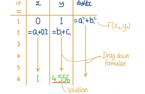
Example Given \( \frac{dy}{dx} = x^2 + y^2 \), and initial point \( (0, 1) \), use a step size of 0.2 to estimate \( y \) when \( x = 1 \) using Euler’s Method. ▶️Answer/ExplanationManual Calculation (Euler’s Method):
Using GDC (TI-nspire Lists & Spreadsheets):
Drag down the formulas and at row 6 (i.e. \( x = 1 \)), the solution is: 4.556 |
Coupled Systems of Differential Equations
A system of differential equations involves more than one dependent variable. A coupled system is where the equations depend on each other.
For example, a system might look like:
$ \begin{cases} \frac{dx}{dt} = f(x, y) \\ \frac{dy}{dt} = g(x, y) \end{cases} $
Such systems arise in real-world scenarios like physics, chemistry, economics, and biology.
Numerical methods like Euler’s Method can be extended to systems:
- Compute \(x_{n+1} = x_n + h \cdot f(x_n, y_n)\)
- Compute \(y_{n+1} = y_n + h \cdot g(x_n, y_n)\)
Spreadsheets can also be used to simulate coupled systems by maintaining separate columns for each variable and its update formula.
Example Consider the system: $ \frac{dx}{dt} = 3x + 4y, \quad \frac{dy}{dt} = -4x + 3y $ ▶️Answer/ExplanationFind eigenvalues of the matrix: $ \begin{bmatrix} 3 & 4 \\ -4 & 3 \end{bmatrix} \Rightarrow \lambda = 3 \pm 4i $] This is a spiral center — solutions rotate and grow. |
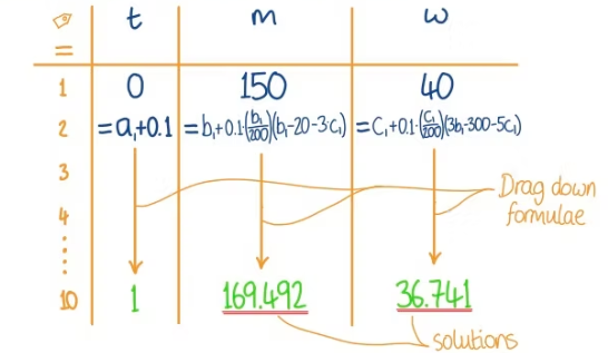
Example The population of moose \( m \) and wolves \( w \) on an island, after \( t \) years, is modeled by the coupled system: $ \frac{dm}{dt} = \frac{1}{200} m (150 – 20 – 3w), \quad \frac{dw}{dt} = \frac{1}{200} w (3m – 300 – 5w) $ Initially, there are 150 moose and 40 wolves. Using a step length of \( h = 0.1 \), estimate the population of moose and wolves after 1 year. ▶️Answer/ExplanationManual Step (Euler’s Method): Let \( m_0 = 150 \), \( w_0 = 40 \) $ \frac{dm}{dt} = \frac{150}{200}(150 – 20 – 3(40)) = \frac{3}{4}(40) = 30 \Rightarrow m_1 = 150 + 0.1 \cdot 7.5 = 150.75$ $\frac{dw}{dt} = \frac{40}{200}(3(150) – 300 – 5(40)) = \frac{1}{5}(-50) = -10 \Rightarrow w_1 = 40 + 0.1(-10) = 39 $ So after \( \frac{1}{10} \) of a year, the populations are approximately \( m = 150.75 \), \( w = 39 \). Using GDC (TI-nspire Lists & Spreadsheets):
Drag down formulas to row 11 (i.e. \( t = 1 \)):
|
Error in Euler’s Method: Local and Global Truncation Errors
Euler’s method is a fundamental numerical approach for approximating solutions to differential equations. However, its simplicity comes at the cost of truncation errors, which arise from approximating the actual curve using straight-line segments.
Local Truncation Error
This refers to the error made during a single step of Euler’s method. It occurs because the method assumes the slope of the solution remains constant over the step interval \( h \), whereas in reality, the slope is changing.
Key property:
Local truncation error is proportional to the square of the step size:
$ \text{Local error} \propto h^2 $
This means reducing the step size significantly lowers the error per step.
Global Truncation Error
Global error is the accumulated error over all steps in the interval. It represents the total deviation from the true solution after many iterations.
Key property:
Global truncation error is proportional to the step size:
$ \text{Global error} \propto h $
If you halve the step size \( h \), the total accumulated error is also approximately halved.
Minimizing Error
- Use a smaller step size \( h \) to reduce both local and global errors.
- Alternatively, use more accurate numerical methods like the Runge–Kutta methods, which provide better accuracy with similar step sizes.
Conclusion: A good understanding of local and global errors allows for an optimal balance between computational cost and desired accuracy when applying Euler’s method.
Example Approximate \( y(1) \) using Euler’s method for \( \frac{dy}{dt} = y \) with \( y(0) = 1 \), step size \( h = 0.5 \). ▶️Answer/ExplanationSteps: $ y_1 = 1 + 0.5(1) = 1.5, \quad y_2 = 1.5 + 0.5(1.5) = 2.25 $ True value: \( e^1 \approx 2.718 \) Global error: \( 2.718 – 2.25 = 0.468 \) Local error occurs at each step and is proportional to \( h^2 \), while global error ∝ \( h \). |