IB Mathematics AI AHL Solutions of second order differential equation MAI Study Notes - New Syllabus

IB Mathematics AI AHL Solutions of second order differential equation MAI Study Notes

LEARNING OBJECTIVE

Euler’s method for second-order differential equations

Key Concepts:

Euler’s method for second-order differential equations
Phase portraits

Converting Second-Order DEs to Systems of First-Order DEs

A second-order differential equation of the form: $ \frac{d^2y}{dt^2} = f(t, y, \frac{dy}{dt}) $ can be rewritten as a system of first-order equations by letting:

$ y_1 = y $ (the original function)
$ y_2 = \frac{dy}{dt} $ (first derivative of $ y $)

Then, we get the system $\begin{cases} \frac{dy_1}{dt} = y_2 \\ \frac{dy_2}{dt} = f(t, y_1, y_2) \end{cases} $ This system can now be solved using Euler’s method.

Example

Convert the equation $ \frac{d^2x}{dt^2} + 4\frac{dx}{dt} + 5x = 0 $ into a system of first-order differential equations.

▶️Answer/Explanation

Let $ x_1 = x $, $ x_2 = \frac{dx}{dt} $.

Then:

$ \frac{dx_1}{dt} = x_2, \quad \frac{dx_2}{dt} = -4x_2 – 5x_1 $

Final system:

$ \begin{cases} \frac{dx_1}{dt} = x_2 \\ \frac{dx_2}{dt} = -4x_2 – 5x_1 \end{cases} $

Euler’s Method for Systems

For a step size $ h $, the Euler updates are:

$ t_{n+1} = t_n + h $
$ y_{1,n+1} = y_{1,n} + h \cdot y_{2,n} $
$ y_{2,n+1} = y_{2,n} + h \cdot f(t_n, y_{1,n}, y_{2,n}) $

Example

Use Euler’s method with step size $ h = 0.1 $ to estimate $ x(0.1) $ and $ v(0.1) $ for $ \frac{d^2x}{dt^2} = -x $, with $ x(0) = 1 $, $ \frac{dx}{dt}(0) = 0 $.

▶️Answer/Explanation

Convert to system variables:

$ x_1 = x, \quad x_2 = \frac{dx}{dt} $ $ \frac{dx_1}{dt} = x_2, \quad \frac{dx_2}{dt} = -x_1 $

Initial conditions:

$ x_1(0) = 1, \quad x_2(0) = 0 $

Apply Euler’s method:

$ x_1(0.1) = 1 + 0.1 \times 0 = 1, \quad x_2(0.1) = 0 + 0.1 \times (-1) = -0.1 $

Approximate values at $ t = 0.1 $:

$ x(0.1) \approx 1, \quad \frac{dx}{dt}(0.1) \approx -0.1 $

Using Spreadsheets (GDC or Excel)

To use a spreadsheet:

Create columns for $ t_n $, $ y_1 $, $ y_2 $, and $ f(t, y_1, y_2) $.
Initialize the first row with given initial values: $ t_0 $, $ y_1(0) $, and $ y_2(0) $.
Use formulas in subsequent rows:
- $ t_{n+1} = t_n + h $
- $ y_{1,n+1} = y_{1,n} + h \cdot y_{2,n} $
- $ y_{2,n+1} = y_{2,n} + h \cdot f(t_n, y_{1,n}, y_{2,n}) $
Drag formulas down to compute the solution over time.

Example

Use a spreadsheet to solve $ \frac{d^2x}{dt^2} = -x $ with initial conditions $ x(0) = 1 $, $ \frac{dx}{dt}(0) = 0 $, step size $ h = 0.1 $.

▶️Answer/Explanation

Spreadsheet setup (columns):

$
\begin{array}{|c|c|c|c|c|}
\hline
t & x & v & \dfrac{dx}{dt} = v & \dfrac{dv}{dt} = -x \\
\hline
0.0 & 1.000 & 0.000 & =C_2 & =-B_2 \\
0.1 & =B_2 + D_2 \cdot 0.1 & =C_2 + E_2 \cdot 0.1 & & \\
\hline
\end{array}
$

At $ t=0.1 $, approximate $ x \approx 1.0 $, $ v \approx -0.1 $.

Physical Phenomena Modeled by Second-Order DEs

Many physical systems are naturally modeled by second-order differential equations. Examples include:

Spring-Mass-Damper Systems: $ m\frac{d^2x}{dt^2} + c\frac{dx}{dt} + kx = 0 $
Free Fall with Air Resistance: $ m\frac{dv}{dt} = mg – kv^2 $
Simple Pendulum: $ \frac{d^2\theta}{dt^2} + \frac{g}{L} \sin(\theta) = 0 $

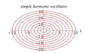
Example

A mass-spring system is modeled by $ \frac{d^2x}{dt^2} + 4x = 0 $. Describe the motion and write the first-order system.

▶️Answer/Explanation

Let $ x_1 = x $, $ x_2 = \frac{dx}{dt} $.

Then:

$ \frac{dx_1}{dt} = x_2, \quad \frac{dx_2}{dt} = -4x_1 $

This describes a harmonic oscillator with periodic oscillations about the equilibrium point.

Phase Portraits and Second-Order Differential Equations

Solutions of second-order differential equations of the form: $ \frac{d^2x}{dt^2} + a \frac{dx}{dt} + b x = 0$ can be investigated using the phase portrait method .

Converting to First-Order System

Define:

$ x_1 = x $
$ x_2 = \frac{dx}{dt} $

Then the system becomes: $ \begin{cases} \frac{dx_1}{dt} = x_2 \\ \frac{dx_2}{dt} = -a x_2 – b x_1 \end{cases}$

Analyzing the Phase Portrait

The phase portrait is a plot of $ x_2 $ (velocity) vs. $ x_1 $ (displacement), and shows the trajectory of the system in phase space. Key behaviors based on values of $ a $ and $ b $:

Underdamped Oscillation: Spiral toward equilibrium (complex roots, Re < 0)
Overdamped Motion: Smooth return to equilibrium (real negative roots)
Critically Damped: Fastest return without oscillation
Unstable Motion: Spiral out or diverging lines (Re > 0)

Why It Matters

Phase portraits provide a powerful visual tool to understand:

Stability of equilibrium points
Oscillations and damping behavior
Long-term system dynamics without solving equations analytically

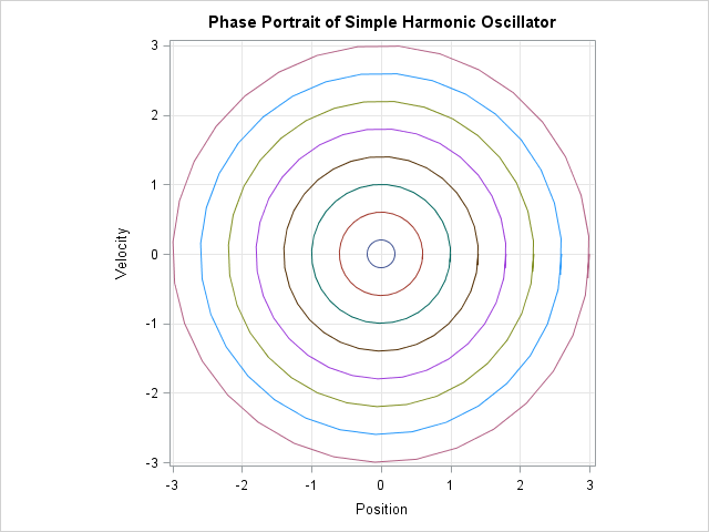
Example

Analyze the phase portrait of the system: $ \frac{dx_1}{dt} = x_2 $, $ \frac{dx_2}{dt} = -x_1 $.

▶️Answer/Explanation

This system represents a simple harmonic oscillator.

The phase portrait consists of closed elliptical orbits around the origin.

The equilibrium at the origin is a center (neutrally stable).

Note: Solutions of $ \frac{d^2x}{dt^2} + a\frac{dx}{dt} + b = 0 $ can also be investigated by phase portraits as covered in AHL 5.17.

Previous Topic Notes

IB Mathematics AI AHL Solutions of second order differential equation MAI Study Notes - New Syllabus

IB Mathematics AI AHL Solutions of second order differential equation MAI Study Notes

EULER’S METHOD FOR SECOND-ORDER DIFFERENTIAL EQUATIONS

PHYSICAL PHENOMENA MODELED AND PHASE PORTRAITS

Resources

Members

Company