IB Mathematics AI AHL Test for proportion MAI Study Notes - New Syllabus
IB Mathematics AI AHL Test for proportion MAI Study Notes
LEARNING OBJECTIVE
- Critical values and critical regions.
Key Concepts:
- Critical values and critical regions.
- Test for population mean for normal/Poisson/Binomial distribution.
- Hypothesis testing
- Type I and II errors
- IBDP Maths AI SL- IB Style Practice Questions with Answer-Topic Wise-Paper 1
- IBDP Maths AI SL- IB Style Practice Questions with Answer-Topic Wise-Paper 2
- IB DP Maths AI HL- IB Style Practice Questions with Answer-Topic Wise-Paper 1
- IB DP Maths AI HL- IB Style Practice Questions with Answer-Topic Wise-Paper 2
- IB DP Maths AI HL- IB Style Practice Questions with Answer-Topic Wise-Paper 3
CRITICAL VALUES AND REGIONS
Critical Values
Boundaries that define the critical (rejection) region in a distribution.
Depend on:
Significance level $(α)$
One-tailed or two-tailed test
Standard Normal Distribution $(z):$
Two-tailed test
$α = 0.05 →$ Critical values: $±1.96$
One-tailed test
$α = 0.05 →$ Critical value: $±1.645$
Critical Region
Range of test statistic values that lead to rejecting the null hypothesis (H₀).
Determined by:
Critical values
Area of critical region $= α$
Cases of $H_1$
1.
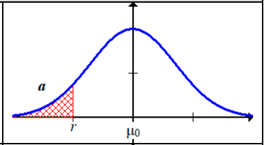
$μ<μ_0$
The red area $X<r$
2.
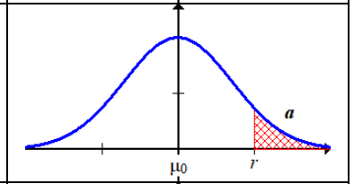
$μ>μ-0$
The red area $X>r$
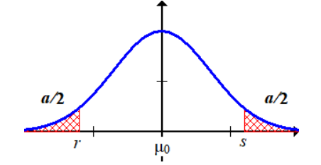
3.
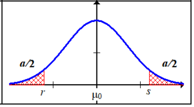
$μ\neq μ_0$
The red area $X<r$ or $X>s$
We will call the remaining region non-critical.
Example For a sample of \( n = 40 \), we know \( \bar{x} = 23 \). We also know that the population standard deviation is \( \sigma = 2.8 \). \( H_0: \mu = 24 \) Find the critical region and the non-critical region. ▶️Answer/ExplanationSolution: (a) Critical and Non-Critical Region:
|
USE OF NORMAL AND T-DISTRIBUTION
Z-Test (Normal Distribution)
Use when $σ$ is known
Applicable regardless of sample size
Formula:
$
z = \frac{\bar{x} – \mu_0}{\sigma / \sqrt{n}}
$
Example For a sample of \( n = 40 \) data (normally distributed), we know that: There is a CLAIM that \( \mu = 24 \).
Use the significance level \( \alpha = 0.05 \) ▶️Answer/ExplanationSolution Since we know \( \sigma \), we use the Z-test (note: \( s_{n-1} = 3 \) was not necessary). Use GDC: Statistics → TEST → Z – 1 SAMPLE → Data: Variable
|
T-Test (t-Distribution)
Use when $σ$ is unknown
Works for any sample size, but especially small samples $(n ≤ 30)$
Formula:
$
t = \frac{\bar{x} – \mu_0}{s / \sqrt{n}}
$
Note:
Use z-test when σ is known, $t-$test when $σ$ is unknown.
Example For a sample of \( n = 20 \) data, we know that: There is a CLAIM that \( \mu = 24 \).
Use the significance level \( \alpha = 0.05 \) ▶️Answer/ExplanationSolution Since we don’t know \( \sigma \), we use the t-test. Use GDC: Statistics → TEST → t – 1 SAMPLE → Data: Variable
|
PAIRED VS. UNPAIRED SAMPLES
Unpaired Samples
Independent groups
Example: Two different classes
Paired Samples
Dependent observations (e.g., before/after)
Analyze the difference
Example: Weight before and after treatment → Paired t-test
| Approach | Design | Type of Data | Appropriate Test |
|---|---|---|---|
| Unpaired Samples | Two different classes of students are randomly assigned: • Class 1 uses Method A • Class 2 uses Method B After teaching, both take the same math test. | Independent groups – different students in each group. | Use an unpaired (independent) t-test Because the groups are unrelated and sampled independently. |
| Paired Samples | The same group of students: • First learns with Method A and takes a test • Then learns with Method B and takes another test | Dependent data – two scores per student (A vs B) | Use a paired t-test Because we compare the same individuals under both conditions. |
TEST FOR PROPORTION
Test for Proportion (Binomial Distribution)
Use when outcomes are binary (success/failure)
Test Statistic:
$
z = \frac{\hat{p} – p_0}{\sqrt{\frac{p_0(1 – p_0)}{n}}}
$
$\hat{p}$: sample proportion
$p_0$: hypothesized proportion
$n$: sample size
Example:
Claim: 80% satisfaction → In a sample of 100, only 75 satisfied → Test with binomial distribution
Example In a sample of 200 people, there are 50 smokers. That is: For the test: \( H_0: p = 0.30 \) Find the critical region and the non-critical region. ▶️Answer/ExplanationSolution We use the distribution \( B(200, 0.30) \) Critical Region :\( X \le 48 \) Non-Critical Region : \( X \ge 49 \) |
Test for Mean Using Poisson Distribution
Use for count data (e.g., defects)
Test Statistic:
$
z = \frac{\bar{x} – \lambda_0}{\sqrt{\lambda_0 / n}}
$
$\bar{x}$: sample mean
$\lambda_0$: hypothesized mean
$n$: number of observations
Example:
Old rate = 2/day, after 10 days observe 15 → Use Poisson test to evaluate change
Testing Correlation Coefficient
Hypothesis:
$ρ = 0$ (no linear correlation)
Test Statistic:
$
t = \frac{r \sqrt{n – 2}}{\sqrt{1 – r^2}} \quad \text{with } (n – 2) \text{ degrees of freedom}
$
Purpose:
Test if there is a significant linear relationship between two variables
Example The number of accidents per day in a certain area follows a Poisson distribution.
The statistic is \( \sum X_i = 39 \) For the test: Find the critical region and the non-critical region. ▶️Answer/ExplanationSolution We use the Poisson distribution \( \text{Po}(35) \) Critical Region : \( X \ge 44 \) Non-Critical Region : \( X \le 43 \) |
TYPE I AND TYPE II ERRORS
Type I
Rejecting $H_0$ when it’s true $α$ (Significance level)
Type II
Failing to reject H₀ when it’s false $β $
Note:
Type I → False positive
Type II → False negative
Probability of Type II Error:
$
\beta = P\left(Z < \frac{z_{\text{crit}} – (\mu – \mu_0)}{\sigma / \sqrt{n}}\right)
$
Example: For a sample of \( n = 40 \), we know \( \bar{x} = 23 \). We also know that the population standard deviation is \( \sigma = 2.8 \). For the test: \( H_0: \mu = 24 \)
▶️Answer/ExplanationSolution: (a) Type I Error: This is the probability of rejecting \( H_0 \) when \( H_0 \) is true. Thus, (b) Type II Error:
|
Example: Context: Heights of 5th graders around the world follow \( X \sim N(142, 5^2) \). You believe students at your school are taller, so you collect a sample of \( n = 32 \) students. After conducting a hypothesis test at a 5% significance level, the true mean is later revealed to be \( \mu = 146 \). Calculate \( P(\text{Type II Error}) \). ▶️ Solution/ExplanationHypotheses $ H_0: \mu = 142 \quad \text{(normal population)} \\ H_1: \mu > 142 \quad \text{(taller than normal)} $ Sampling Distribution under \( H_0 \) The sample mean \( \bar{X} \sim N\left(142, \frac{25}{32} \right) \), since \( \sigma^2 = 5^2 = 25 \). Standard error: $ \text{SE} = \sqrt{\frac{25}{32}} \approx 0.990 $ Step 3: Critical Value (C.V.) for 5% significance level (1-tailed test) We find the value of \( \bar{x} \) such that: $ P(\bar{X} \leq \text{C.V.}) = 0.95 \quad \text{(because upper 5% is rejection region)} $ Using: $ \text{C.V.} = \text{invNorm}(0.95, 142, 0.990) \approx 143.74 $ Type II Error Type II error is the probability of failing to reject \( H_0 \) when \( \mu = 146 \) is true: Under \( \mu = 146 \), the distribution of \( \bar{X} \sim N(146, 0.990) \). So, $ P(\text{Type II Error}) = P(\bar{X} \leq 143.74 \mid \mu = 146) = \text{normalcdf}(-\infty, 143.74, 146, 0.990) \approx 0.0166 $ Conclusion: There is a 1.66% chance of failing to detect that the students are taller than normal. This is the probability of a Type II error for a sample of size 32. |
DISCRETE DISTRIBUTIONS AND ONE-TAILED TESTS
IB only requires one-tailed tests for discrete distributions (binomial, Poisson). Define critical region to maximize Type I error without exceeding $α$
Assumptions for Hypothesis Tests
Before performing a hypothesis test, certain assumptions must be satisfied to ensure the validity of the results.
Z-Test Assumptions
- The population is normally distributed, or the sample size is large enough (typically $n ≥ 30$) for the Central Limit Theorem to apply.
- The population standard deviation ($σ$) is known.
- The data points are independent (no dependence between observations).
T-Test Assumptions
- The population is normally distributed — this is especially important when the sample size is small (typically $n ≤ 30$).
- The population standard deviation (σ) is unknown, and is estimated using the sample standard deviation (s).
- The data points are independent.