Home / IB DP Maths 2026, 2027 & 2028 / Application and Interpretation HL / IB Mathematics AI AHL The second derivative MAI Study Notes

IB Mathematics AI AHL The second derivative MAI Study Notes - New Syllabus

IB Mathematics AI AHL The second derivative MAI Study Notes

LEARNING OBJECTIVE

  • The second derivative.

Key Concepts: 

  • The second derivative.
  • Use of second derivative.

MAI HL and SL Notes – All topics

 THE SECOND DERIVATIVE 

 The Second Derivative 

The second derivative of a function provides information about the curvature or concavity of the graph.

If a function is \( f(x) \), its second derivative is denoted as:

\( \frac{d^2y}{dx^2} \) or \( f”(x) \)

The second derivative is simply the derivative of the first derivative:

\( f”(x) = \frac{d}{dx}\left( \frac{dy}{dx} \right) \)

It tells us how the rate of change is itself changing.

Example : 

Identify the local maximum or minimum for the function: \( f(x) = x^3 – 6x^2 + 9x + 1 \)

▶️Answer/Explanation
  • \( f'(x) = 3x^2 – 12x + 9 \)
  • Set derivative to zero: \( 3x^2 – 12x + 9 = 0 \Rightarrow x = 1, 3 \)
  • \( f”(x) = 6x – 12 \)
  • \( f”(1) = -6 \lt 0 \Rightarrow \) local maximum at \( x = 1 \)
  • \( f”(3) = 6 \gt 0 \Rightarrow \) local minimum at \( x = 3 \)

CONCAVITY, SECOND DERIVATIVE TEST & POINTS OF INFLEXION 

Concavity

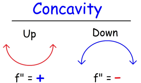
Concavity describes the shape of the curve. If the average rates are increasing on an interval then the function is concave up and if the average rates are decreasing on an interval then the function is concave down on the interval.

  • If \( f”(x) > 0 \), the curve is concave up (“smile”).
  • If \( f”(x) < 0 \), the curve is concave down (“frown”).

Example : 

Determine intervals of concavity for the function: \( f(x) = x^4 – 4x^3 \)

▶️Answer/Explanation
  • \( f'(x) = 4x^3 – 12x^2 \)
  • \( f”(x) = 12x^2 – 24x \)
  • Set \( f”(x) = 0 \Rightarrow 12x(x – 2) = 0 \Rightarrow x = 0, 2 \)
  • Test intervals:
    • \( x < 0 \Rightarrow f”(x) > 0 \Rightarrow \) concave up
    • \( 0 < x < 2 \Rightarrow f”(x) < 0 \Rightarrow \) concave down
    • \( x > 2 \Rightarrow f”(x) > 0 \Rightarrow \) concave up
  • Therefore, \( x = 0 \) and \( x = 2 \) are points of inflexion.

Second Derivative Test for Turning Points:

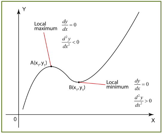
Suppose \( f'(x) = 0 \) at \( x = a \):

  • If \( f”(a) > 0 \), there is a local minimum.
  • If \( f”(a) < 0 \), there is a local maximum.
  • If \( f”(a) = 0 \), the test is inconclusive.

Identifying Maximum and Minimum Points

To find local maxima or minima:

  1. Solve \( f'(x) = 0 \) to find critical points.
  2. Apply the second derivative test:
    • If \( f”(x) > 0 \), it’s a minimum.
    • If \( f”(x) < 0 \), it’s a maximum.
    • If \( f”(x) = 0 \), test is inconclusive — use a sign chart or first derivative test.

Point of Inflexion:

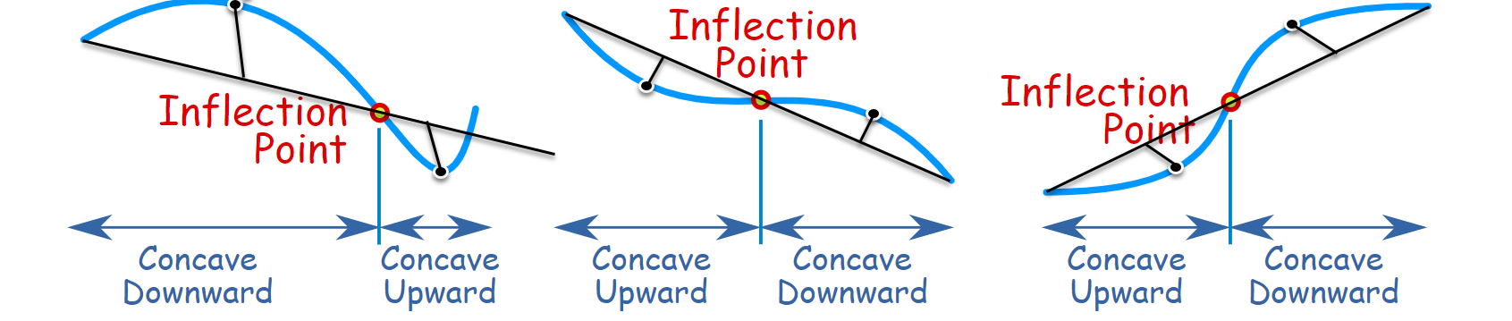
A point where concavity changes from up to down (or vice versa). At such a point:

    • \( f”(x) = 0 \) and the sign of \( f”(x) \) changes.

Example : 

Find and classify critical points for: \( f(x) = \ln(x^2 + 1) \)

▶️Answer/Explanation
  • \( f'(x) = \frac{2x}{x^2 + 1} \)
  • Set \( f'(x) = 0 \Rightarrow x = 0 \)
  • \( f”(x) = \frac{2(x^2 + 1) – 4x^2}{(x^2 + 1)^2} = \frac{2 – 2x^2}{(x^2 + 1)^2} \)
  • \( f”(0) = \frac{2}{1} = 2 \gt 0 \Rightarrow \) local minimum at \( x = 0 \)

LINKS TO OTHER TOPICS 

Kinematics (AHL 5.13):

In physics, the position of an object as a function of time is given by \( s(t) \). The second derivative \( s”(t) \) represents the object’s acceleration, which is the rate of change of velocity. This helps in understanding motion — whether an object is speeding up or slowing down.

Example (Kinematics):

Let \( s(t) = 4t^3 – 3t^2 + 2t \)

▶️Answer/Explanation
  • Velocity: \( v(t) = s'(t) = 12t^2 – 6t + 2 \)
  • Acceleration: \( a(t) = s”(t) = 24t – 6 \)

Second-order Differential Equations (AHL 5.18):

Many physical systems like springs, pendulums, and electric circuits involve oscillatory motion, which is modeled using second-order differential equations. These often take the form \( \frac{d^2y}{dt^2} + a\frac{dy}{dt} + by = 0 \). The second derivative shows how acceleration or force acts over time to influence motion.

Example (Second-Order Differential Equation):

Consider \( \frac{d^2y}{dt^2} + 4y = 0 \)

▶️Answer/Explanation
  • This is a simple harmonic oscillator.
  • General solution: \( y(t) = A\cos(2t) + B\sin(2t) \)
  • Where A and B are constants determined by initial conditions.
Scroll to Top