IB Mathematics AI AHL Transition matrices. MAI Study Notes- New Syllabus

IB Mathematics AI AHL Transition matrices. MAI Study Notes

LEARNING OBJECTIVE

Transition matrices.

Key Concepts:

Transition matrices.
Powers of transition matrices.
Regular Markov chains & Initial state probability matrices.
Eigenvalue Condition for Steady State

A transition matrix, also known as a state transition matrix or Markov matrix, is a square matrix used to represent the probabilities of transitioning between different states in a system. Each element in the matrix represents the probability of moving from one state (represented by a row) to another state (represented by a column).

A transition matrix represents the probabilities of moving between different states in a Markov system or stochastic process.

Rows = Next state (i.e. destination)
Columns = Current state (i.e. origin)
Entries = Probability of transitioning from the current state to the next
Each column must sum to 1 (since total probability of leaving a state is 1)

Key Features:

All entries must be between 0 and 1.
The matrix is often square: if there are $ n $ states, the matrix is $ n \times n $.
Used to model systems evolving over discrete time steps.
Common in population models, economics, genetics, and game theory.

Example

Population Movement Between Two Cities

From A: 80% stay, 20% move to B
From B: 70% stay, 30% move to A

Find the Transition Matrix

▶️ Answer/Explanation

Let the states be:

State A
State B

Transition Matrix $ T $:

$ T = \begin{pmatrix} 0.8 & 0.3 \\ 0.2 & 0.7 \end{pmatrix} $

Each column represents the current state (A, B).
Each row represents the next state.
Each column sums to 1: $ 0.8 + 0.2 = 1 $, $ 0.3 + 0.7 = 1 $.

Powers of a Transition Matrix

To find the probability distribution after multiple steps, we raise the transition matrix to a power:

$ T^n $ gives the probabilities of transitioning between states after n time steps.

Why use powers?

$ T^2 $: shows 2-step transition probabilities
$ T^3 $: shows 3-step transitions, and so on
Multiplying the matrix by an initial state vector gives the system’s state at the next step

Example

Use the matrix from the previous example:
From A: 80% stay, 20% move to B
From B: 70% stay, 30% move to A

Find the probability of being in each city after 2 steps.

▶️ Answer/Explanation

Given Transition Matrix $ T $:

$ T = \begin{pmatrix} 0.8 & 0.3 \\ 0.2 & 0.7 \end{pmatrix} $

Find $ T^2 $ to get the 2-step transition matrix:

$ T^2 = T \cdot T = \begin{pmatrix} 0.8 & 0.3 \\ 0.2 & 0.7 \end{pmatrix} \cdot \begin{pmatrix} 0.8 & 0.3 \\ 0.2 & 0.7 \end{pmatrix} $

$ = \begin{pmatrix} (0.8)(0.8)+(0.3)(0.2) & (0.8)(0.3)+(0.3)(0.7) \\ (0.2)(0.8)+(0.7)(0.2) & (0.2)(0.3)+(0.7)(0.7) \end{pmatrix} $

$ = \begin{pmatrix} 0.70 & 0.45 \\ 0.30 & 0.55 \end{pmatrix} $

The matrix $ T^2 $ gives probabilities after 2 transitions.
For example: If starting in A, the probability of being in A after 2 steps is 0.70.

Transition Diagrams in Discrete Dynamical Systems

Definition: A transition diagram is a directed graph that visually represents the movement between states in a system. It is commonly used with transition matrices in discrete dynamical systems.

Key Features:

Nodes: Represent the different states in the system.
Arrows: Show the direction of transition from one state to another.
Weights on arrows: Indicate the probability or proportion of moving from one state to the next.
Used with: Transition matrices $ T $, where entries $ T_{ij} $ represent the probability of moving from state $ j $ to state $ i $.

Connection to Transition Matrices:

Each column in the transition matrix corresponds to a state you are moving from, and each row shows the state you are moving to.

Use in Dynamical Systems:

If the initial state is given by a column vector (e.g. $ \begin{pmatrix} 100 \\ 0 \end{pmatrix} $), then repeated multiplication by the transition matrix will simulate how populations evolve over time:

$ \text{Next state} = T \times \text{Current state} $ $ \text{After } n \text{ steps: } \quad \mathbf{x}_n = T^n \cdot \mathbf{x}_0 $

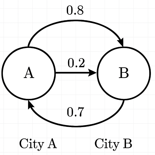
Example:

Consider two cities, A and B:

From A: 80% stay in A, 20% move to B
From B: 70% stay in B, 30% move to A

From \ To	City A	City B
City A	0.8	0.3
City B	0.2	0.7

Find Transition Matrix and describe Transition Diagram:

▶️ Answer/Explanation

Solution:

Transition Matrix:

$T = \begin{pmatrix} 0.8 & 0.3 \\ 0.2 & 0.7 \end{pmatrix} $

Transition Diagram:

Draw two circles labeled A and B.
From A, draw an arrow looping back to A labeled 0.8, and an arrow to B labeled 0.2.
From B, draw an arrow looping back to B labeled 0.7, and an arrow to A labeled 0.3.

A Markov Chain is a model for a system that transitions between states with fixed probabilities.

Key Property – Memorylessness:

The probability of moving to the next state depends only on the current state, not on the sequence of previous states.

Terminology:

States: The different conditions a system can be in
Transitions: Movements between states with associated probabilities
Transition Matrix: Encodes all transition probabilities

State Vector $S_n$:

Represents the distribution of the system at time $n$.

Each entry gives the number (or probability) of people/items in each state.

Updating State Vectors:

$
S_{n+1} = T \times S_n
$

Or recursively:

$
S_n = T^n \times S_0
$

Example

Let:

$
S_0 = \begin{pmatrix} 50 \\ 50 \end{pmatrix}
\quad \text{(50 in A, 50 in B)}
$

Find

$S_1:?$

▶️Answer/Explanation

Solution:

$
S_1 = T \times S_0 = \begin{pmatrix} 0.8 & 0.3 \\ 0.2 & 0.7 \end{pmatrix} \begin{pmatrix} 50 \\ 50 \end{pmatrix} = \begin{pmatrix} 55 \\ 45 \end{pmatrix}
$

$
S_2 = T^2 \times S_0 = \begin{pmatrix} 0.70 & 0.45 \\ 0.30 & 0.55 \end{pmatrix} \begin{pmatrix} 50 \\ 50 \end{pmatrix} = \begin{pmatrix} 57.5 \\ 42.5 \end{pmatrix}
$

Steady State Vector $S_\infty$:

The long-term behavior of the system as $n \to \infty$:

$
T \times S = S \quad \text{(i.e., eigenvector with eigenvalue 1)}
$

To find:

Solve:

$
\begin{cases}
0.8x + 0.3y = x \\
0.2x + 0.7y = y \\
x + y = 100
\end{cases}
\quad \Rightarrow S_\infty = \begin{pmatrix} 60 \\ 40 \end{pmatrix}
$

Interpretation: Eventually, 60% of people reside in A and 40% in B, regardless of the initial distribution.

Properties of a Steady State Vector

Stationary:

Once reached, applying the transition matrix does not change the vector: $T \times S_\infty = S_\infty$

Unique (under conditions):

If the matrix is regular (some power of $T$ has all positive entries), the steady state is unique.

Independent of Initial State:

Given enough time, the system always tends toward the same steady state, regardless of $S_0$.

Entries Sum to 1 or Total Population:

When working with probabilities, the sum of entries = 1
When using absolute counts, the sum = total population

Represents Long-Term Probabilities:

Each entry gives the long-run proportion of time the system spends in each state. Markov Chains and Long-Term Behavior

Repeated Transitions:

Continue multiplying by the transition matrix.
The system tends to stabilize if a steady state exists.

Applications:

Predict long-term population distributions
Model absorbing or recurrent states
Understand system stability or fluctuations

Example

Positions: 1, 2, 3, 4

At positions 1 & 4 → stops
At 2 or 3 →

Move right: 0.6
Move left: 0.4

Long-Term: ?

▶️Answer/Explanation

Solution:

Transition Matrix $T$:

$
T = \begin{pmatrix}
1 & 0.4 & 0 & 0 \\
0 & 0 & 0.4 & 0 \\
0 & 0.6 & 0 & 0 \\
0 & 0 & 0.6 & 1 \\
\end{pmatrix}
$

Initial State:

$
S_0 = \begin{pmatrix} 0 \\ 1 \\ 0 \\ 0 \end{pmatrix} \quad \text{(starts at position 2)}
$

After 2 Steps:

$
S_2 = T^2 \times S_0 = \begin{pmatrix} 0.40 \\ 0.24 \\ 0 \\ 0.36 \end{pmatrix}
$

Interpretation:

40% chance at position 1
24% chance at position 2
36% chance at position 4

Long-Term:

The robot will eventually stop at position 1 $\rightarrow 52.6\%$ or 4 $\rightarrow 47.4\%$

The steady state of a Markov chain is directly linked to eigenvectors of its transition matrix.

For a transition matrix $ T $, the steady state vector $ S $ satisfies:

$T \times S = 1 \times S$

This means:

$ S $ is an eigenvector of $ T $.
The corresponding eigenvalue is 1.

(Every stochastic matrix $ T $ has at least one eigenvalue equal to 1.)

Finding the Steady State

Given transition matrix for city populations:

$
T = \begin{pmatrix} 0.8 & 0.3 \\ 0.2 & 0.7 \end{pmatrix}
$

using (Eigenvector Method)

▶️Answer/Explanation

Solution:

Solve for eigenvalues $ \lambda $:
$
\det(T – \lambda I) = 0 \implies \begin{vmatrix} 0.8 – \lambda & 0.3 \\ 0.2 & 0.7 – \lambda \end{vmatrix} = 0
$
$
(0.8 – \lambda)(0.7 – \lambda) – (0.3 \times 0.2) = 0 \implies \lambda^2 – 1.5\lambda + 0.5 = 0
$
$
\lambda = 1 \quad \text{or} \quad \lambda = 0.5
$

For $ \lambda = 1 $, eigenvector $ S = \begin{pmatrix} x \\ y \end{pmatrix} $:
$
(T – I)S = 0 \implies \begin{pmatrix} -0.2 & 0.3 \\ 0.2 & -0.3 \end{pmatrix} \begin{pmatrix} x \\ y \end{pmatrix} = \begin{pmatrix} 0 \\ 0 \end{pmatrix}
$
$
-0.2x + 0.3y = 0 \implies 2x = 3y \implies \frac{x}{y} = \frac{3}{2}
$
Thus, the general eigenvector is:
$
S = t \begin{pmatrix} 3 \\ 2 \end{pmatrix}
$

Normalize for total population (e.g., 100 people):
$
3t + 2t = 100 \implies t = 20 \implies S = \begin{pmatrix} 60 \\ 40 \end{pmatrix}
$

(This matches our earlier steady state!)

Interpretation