Home / IB DP Maths 2026, 2027 & 2028 / Application and Interpretation HL / IB Mathematics AI SL Trapezoidal Rule MAI Study Notes

IB Mathematics AI SL Trapezoidal Rule MAI Study Notes - New Syllabus

IB Mathematics AI SL Trapezoidal Rule MAI Study Notes

LEARNING OBJECTIVE

  • Approximating areas using the trapezoidal rule.

Key Concepts: 

  • Trapezoidal rule.

MAI HL and SL Notes – All topics

APPROXIMATING AREAS USING THE TRAPEZOIDAL RULE

 Definition

The trapezoidal rule is a method for estimating the area under a curve (i.e., the definite integral of a function) by dividing the interval into sub-intervals of equal width and approximating the area using trapezoids instead of rectangles.
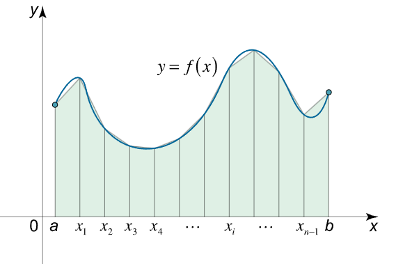
Concept

Suppose we want to estimate the area under the curve \( y = f(x) \) from \( x = a \) to \( x = b \). The interval is divided into \( n \) sub-intervals of equal width \( h = \frac{b – a}{n} \), and the area under the curve is approximated by summing the areas of the trapezoids formed under each subinterval.

Formula

The Trapezoidal Rule approximation for the area is given by:

$ \text{Area} \approx \frac{h}{2} \left[ f(x_0) + 2f(x_1) + 2f(x_2) + \dots + 2f(x_{n-1}) + f(x_n) \right] $

$\int_a^b f(x) \, dx \approx \frac{h}{2} \left[ f(x_0) + 2f(x_1) + 2f(x_2) + \cdots + 2f(x_{n-1}) + f(x_n) \right]$

Where:

  • \( h = \frac{b – a}{n} \) is the width of each subinterval.
  • \( x_0, x_1, \dots, x_n \) are the endpoints of the subintervals (with \( x_0 = a \), \( x_n = b \)).

Accuracy Tip

The more subintervals \( n \) used, the more accurate the estimate will be. If the curve is concave up or down over the interval, the trapezoidal rule may slightly over- or underestimate the area.

Example

Estimate the area under the curve \( f(x) = \ln(x+1) \) from \( x = 0 \) to \( x = 4 \) using 4 equal intervals (i.e., \( n = 4 \)).

▶️Answer/Explanation
    • We have \( a = 0 \), \( b = 4 \), \( n = 4 \), so \( h = \frac{4-0}{4} = 1 \)
    • Compute values:
      • \( f(0) = \ln(1) = 0 \)
      • \( f(1) = \ln(2) ≈ 0.6931 \)
      • \( f(2) = \ln(3) ≈ 1.0986 \)
      • \( f(3) = \ln(4) ≈ 1.3863 \)
      • \( f(4) = \ln(5) ≈ 1.6094 \)
    • Apply trapezoidal rule:

$ \text{Area} ≈ \frac{1}{2} [0 + 2(0.6931 + 1.0986 + 1.3863) + 1.6094] $

$= \frac{1}{2} [0 + 2(3.178) + 1.6094] = \frac{1}{2} [6.356 + 1.6094] = \frac{1}{2} \cdot 7.9654 = 3.9827 $

  • Estimated Area ≈ 3.9827

TRAPEZOIDAL RULE IN TABULAR DATA

 Concept

When a function is not known explicitly but values of \( f(x) \) are given in a table at equally spaced intervals, the trapezoidal rule can still be applied to estimate the area under the curve.

 Formula (Tabular Form)

Given values of \( f(x) \) at \( x_0, x_1, \dots, x_n \) with equal spacing \( h \), the area is estimated using:

$ \text{Area} \approx \frac{h}{2} \left[ y_0 + 2y_1 + 2y_2 + \dots + 2y_{n-1} + y_n \right] $

Where:

  • \( y_i = f(x_i) \)
  • \( h \) is the common interval between successive \( x \)-values.

Example

The table below shows the speed (in m/s) of a car at intervals of 2 seconds. Estimate the distance travelled over the 10 seconds using the trapezoidal rule.

Time (s)Speed (m/s)
$0$$0$
$2$$6$
$4$$10$
$6$$14$
$8$$18$
$10$$20$
▶️Answer/Explanation

There are 6 data points, so \( n = 5 \) intervals. The interval width is \( h = 2 \).

Apply the trapezoidal rule:

$\text{Distance} \approx \frac{2}{2} [0 + 2(6 + 10 + 14 + 18) + 20] $

$= 1[0 + 2(48) + 20] = 1[96 + 20] = \rm{116 \text{ m}}$

Estimated distance travelled = 116 m.

 Connection to Other Topics

Upper and Lower Bounds :

  • The trapezoidal rule provides an approximation that lies between upper and lower Riemann sums depending on the concavity of the function.
  • If the function is concave up, the trapezoidal approximation provides an upper bound for the true area.
  • If the function is concave down, it provides a lower bound.

Area under Curves:

  • The rule is a numerical method for estimating definite integrals when an exact antiderivative may not be known or when data is only available in discrete form.

 Accuracy Tip

The more subintervals \( n \) used, the more accurate the estimate will be. If the curve is concave up or down over the interval, the trapezoidal rule may slightly over- or underestimate the area.

APPLICATION OF THE TRAPEZOIDAL RULE

 Applications in Physics and Real-World Scenarios (Kinematics in Physics)

The trapezoidal rule is widely used in physics, especially when dealing with data from experiments or motion sensors.

  • Distance from Speed-Time Graph: The area under a speed-time graph represents distance travelled.
  • When speed is measured at regular time intervals but not given as a function, trapezoidal rule provides a quick estimate of distance.

Formula: For equally spaced time intervals \( h \),

$ \text{Distance} \approx \frac{h}{2} [v_0 + 2v_1 + 2v_2 + \cdots + 2v_{n-1} + v_n] $

Here \( v_i \) represents the speed at time \( t_i \).

Example: Kinematics – Distance from Speed-Time Table

A car’s speed was recorded every 2 seconds over a 10-second period. Estimate the total distance travelled using the trapezoidal rule.

Time (s):    $0$  $2$  $4$  $6$  $8$  $10$

Speed (m/s):   $0$  $3$  $7$  $6$  $4$  $2$

▶️Answer/Explanation
  • Step 1: Interval width \( h = 2 \) seconds (equal spacing).
  • Step 2: Use the trapezoidal rule formula for tabular data:
  • $ \text{Distance} \approx \frac{h}{2} \left[v_0 + 2v_1 + 2v_2 + 2v_3 + 2v_4 + v_5\right] $
  • $ \text{Distance} \approx \frac{2}{2} \left[0 + 2(3) + 2(7) + 2(6) + 2(4) + 2\right] $
  •  $ = 1 \cdot [0 + 6 + 14 + 12 + 8 + 2] = 1 \cdot 42 = \boxed{42 \text{ m}} $

 So, the estimated distance travelled by the car over 10 seconds is 42 meters.

Irregular Areas

The trapezoidal rule is also useful when estimating areas of irregular shapes, such as:

  • Cross-sections of rivers or lakes
  • Land survey data where exact curve equations are unavailable
  • Engineering curves with known discrete coordinates

In these cases, use tabulated data of coordinates and apply trapezoidal rule on adjacent segments to approximate the total area.

 Using Dynamic Graphing Software

Technology such as GeoGebra, Desmos, and GDCs (Graphical Display Calculators) can visualize the trapezoidal approximation by plotting trapezoids under the curve.

  • These tools help learners better understand how trapezoidal approximation works visually.
  • They can dynamically change the number of intervals and see how increasing intervals leads to better approximations.

Key Benefits:

  • Visual understanding of under- and over-approximation
  • Fast and accurate estimates for real-time applications
  • Interactive learning of numerical integration
Scroll to Top