◆ LIMITS
Limits describe the behavior of a function as the input approaches a certain value.
ESTIMATING LIMITS FROM TABLES AND GRAPHS
- Use values close to the target \(x\) to estimate \(\lim_{x \to c} f(x)\).
- Graphically, observe the \(y\)-value as the curve approaches \(x = c\) from both left and right.
- A limit exists only if both sides approach the same value.
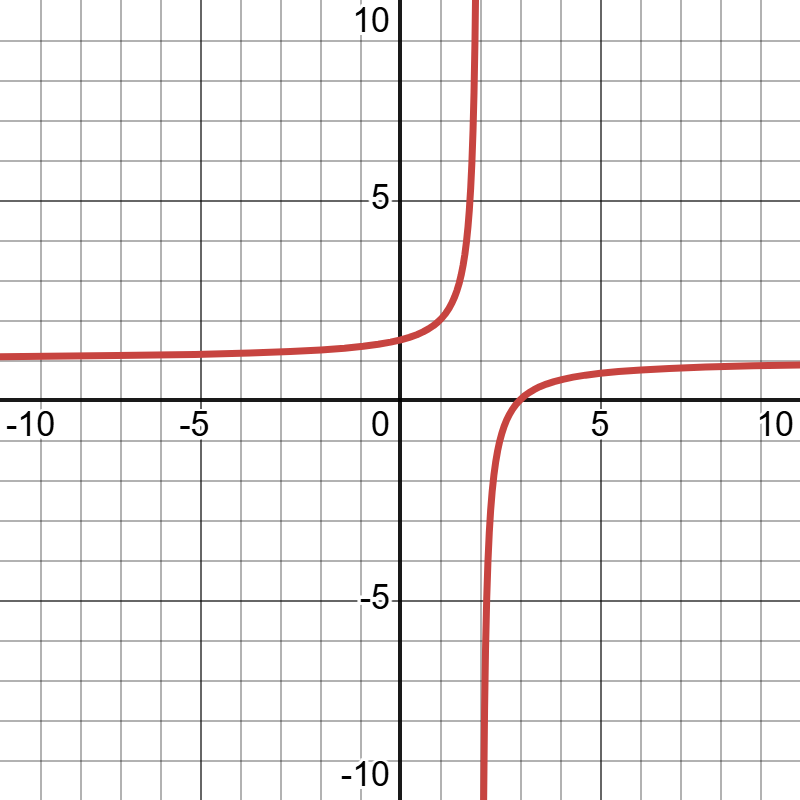
Example (Using graph) Given the function $f(x) = \frac{x – 3}{x – 2}$, identify the vertical and horizontal asymptotes. Also, provide the formal limit-based explanation for each asymptote.
▶️Answer/ExplanationSolution:
Vertical Asymptote: Formal Explanation: $ Horizontal Asymptote: Formal Explanation: $ |
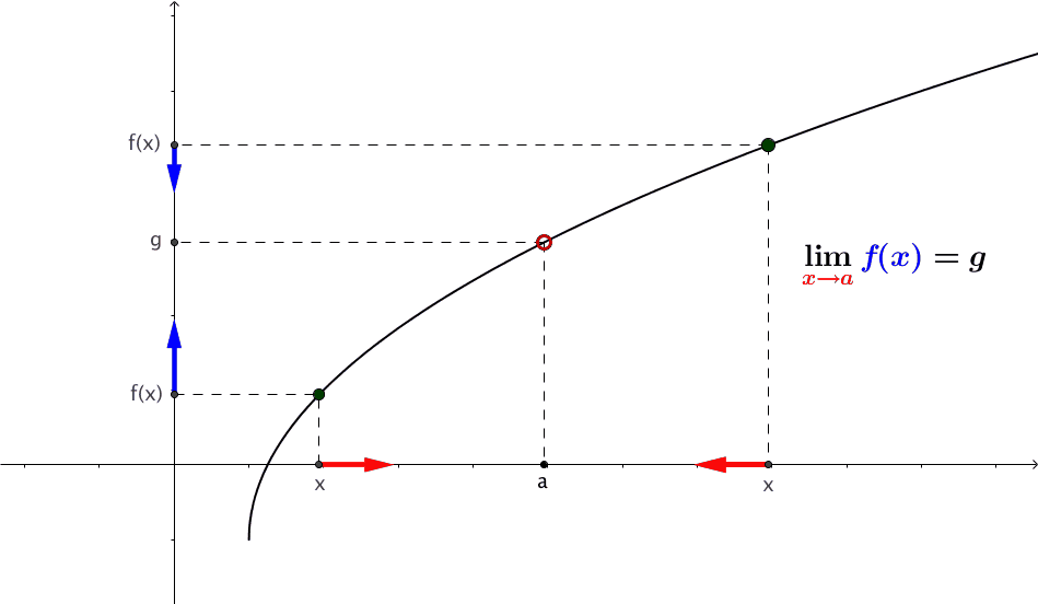
INFORMAL LIMIT NOTATION
\(\lim_{x \to c} f(x) = L\)
- This means that as \(x\) approaches \(c\), \(f(x)\) gets arbitrarily close to \(L\).
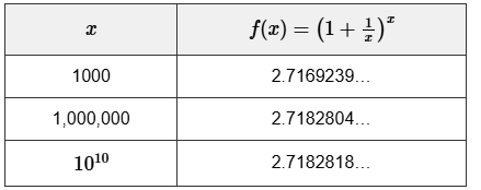
Example (Using table) Investigate the limit $\lim_{x \to \infty} \left(1 + \frac{1}{x} \right)^x$ informally using a calculator. What value does this limit approach? ▶️Answer/ExplanationSolution:
Using values of $x$ approaching infinity: The resulting limit is in fact the number: $ So we conclude: $ |
Example:
Function: \( f(x) = \dfrac{x^2 – 4}{x – 2} \)
Estimate: \( \displaystyle \lim_{x \to 2} f(x) \) using values of \(x\) close to 2.
| x | f(x) |
|---|---|
| 1.9 | 3.9 |
| 1.99 | 3.99 |
| 2.01 | 4.01 |
| 2.1 | 4.1 |
▶️ Answer/Explanation
Solution:
\( f(x) = \frac{x^2 – 4}{x – 2} = \frac{(x – 2)(x + 2)}{x – 2} = x + 2 \), for \( x \ne 2 \).
Conclusion: As \( x \to 2 \), the function values approach 4.
Therefore,
\( \displaystyle \lim_{x \to 2} \frac{x^2 – 4}{x – 2} = 4 \)
Note: The limit exists even though the function is undefined at \( x = 2 \).
INTERPRETING DERIVATIVES AS SLOPES
The derivative at a point gives the slope of the tangent line to the curve at that point.
It represents the instantaneous rate of change of the function.
\( f'(x) = \lim_{h \to 0} \frac{f(x + h) – f(x)}{h} \)
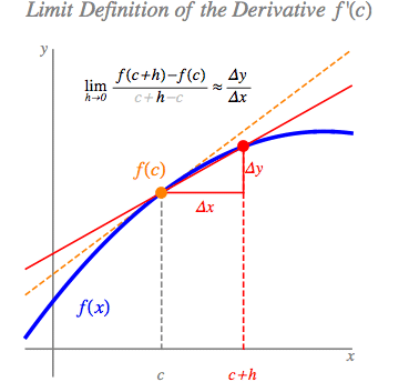
A graph showing a curve with a tangent line at a specific point, illustrating the derivative as the slope of this line
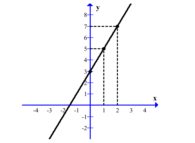
Example : (GRADIENT) ΙΝ Α LINE Consider the line \( f(x) = 2x + 3 \). What is the rate of change (gradient) of this line, and how can it be confirmed using different points on the line? ▶️ Answer/ExplanationSolution:
|
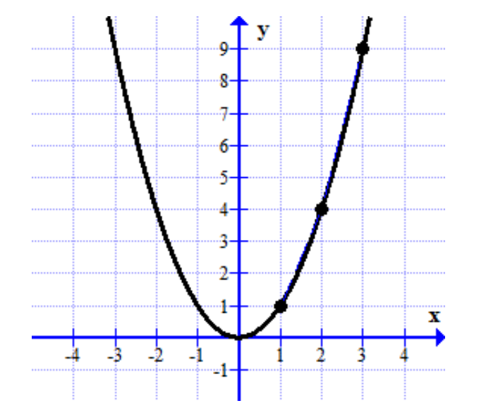
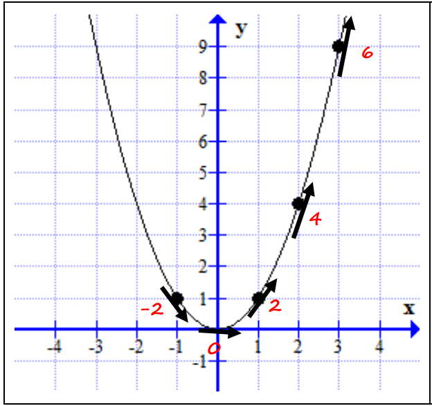
Example : (GRADIENT) ΙΝ Α CURVE In a curve which is not a straight line, the rate of change between any two points is not always the same. For example, consider the function \( f(x) = x^2 \). ▶️ Answer/ExplanationSolution:
However, we can also measure the instantaneous rate of change at a single point — this is the gradient (derivative) at that point.
|
BASIC NOTATIONS FOR DERIVATIVES
- \(\frac{dy}{dx}\): Rate of change of \(y\) with respect to \(x\).
- \(f'(x)\): Derivative of the function \(f\) at \(x\).
- \(\frac{ds}{dt}\): Rate of change of \(s\) with respect to \(t\).
Example Question: If \(s(t) = 5t^3\), find \(\frac{ds}{dt}\). ▶️Answer/Explanation\(\frac{ds}{dt} = 15t^2\) |
NOTATIONS FOR DERIVATIVES
LEIBNIZ NOTATION
- Emphasizes the derivative as the ratio of infinitesimal changes.
- Written as: \(\frac{dy}{dx}, \frac{ds}{dt}\)
LAGRANGE NOTATION
- Often used for simplicity when the function is expressed explicitly in terms of \(x\).
- Written as: \(f'(x), V'(r)\)
Example Question: For \(y = x^2\), write the derivative in both Leibniz and Lagrange notations. Also, for \(V = \pi r^2 h\), find \(\frac{dV}{dr}\). ▶️Answer/Explanation\(\frac{dy}{dx} = 2x\) (Leibniz notation) \(f'(x) = 2x\) (Lagrange notation) \(\frac{dV}{dr} = 2\pi rh\) \(V'(r) = 2\pi rh\) |