When data spans a very large or very small range, plotting it on a linear scale can make trends difficult to see. A logarithmic scale solves this by plotting the logarithm of values instead of the raw values themselves.
Why use logarithmic scales?
Makes it easier to visualize exponential growth or decay
Compresses large numbers and spreads out smaller numbers
Useful for data involving powers of 10, such as:
Earthquake magnitudes (Richter scale)
Sound intensity (decibels)
pH levels
Population growth or radioactive decay
How it works:
In a log scale:
Equal distances on the axis represent equal ratios, not differences.
For example, on a base-10 log scale:
The distance between 1 and 10 is the same as between 10 and 100.
Each tick increases by a factor of 10.
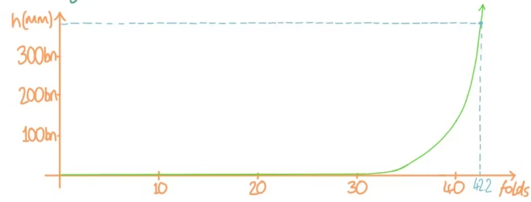
Example A piece of paper is 0.075 mm. We fold it repeatedly (beyond the usual limit of 7). Use a graph to find when it becomes 1 cm thick, then how many folds until it reaches the moon? ▶️Answer/ExplanationSolution: We graph $h(n) = 0.075(2^n)$; Moon $≈ 42$ folds
|
Consider the logarithmic model:
\( y = a + b \ln x \).
If we set \( X = \ln x \), the model takes the form: \( y = a + bX \) [linear].
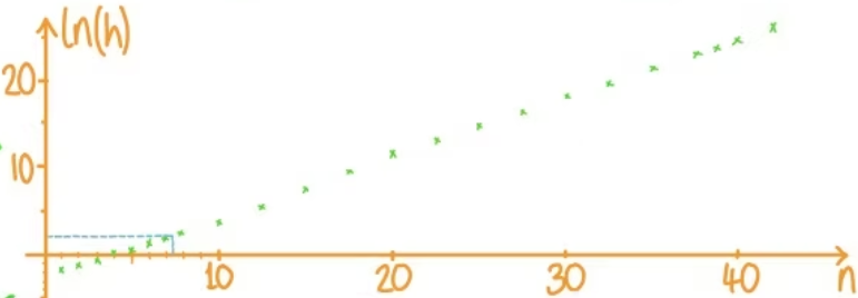
Example Graph the height of the paper against no. of folds on a ln(h) against n graph:
▶️Answer/ExplanationSolution: We need to take each h, and do ln(h)
|
LINEARISATION OF THE EXPONENTIAL MODEL
Consider the exponential model: \( y = Ae^{kx} \).
Apply \( \ln \): \( \ln y = \ln A + kx \).
If we set \( Y = \ln y \), the model takes the form: \( Y = \ln A + kx \) [linear].
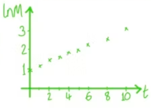
Example For the following data, showing the mass of bacteria (M, grams) after t hours, show that it should fit an exponential model, giving the equation for M in terms of t:
▶️Answer/ExplanationSolution: Semi-log graph:
On GDC, we find a ln(M) column:
Very close to linear, so the original data is exponential. GDC also shows: $m = 0.2065$ Thus: $ $ $ Conclusion: |
LINEARISATION OF THE POWER FUNCTION MODEL
Consider the power function model: \( y = kx^n \).
Apply \( \ln \): \( \ln y = \ln k + n \ln x \).
If we set \( X = \ln x \) and \( Y = \ln y \), it takes the form: \( Y = \ln k + nX \) [linear].
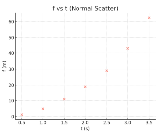
Example A group of students try to model the motion of a football being dropped off their HS roof terrace
▶️Answer/ExplanationSolution: Normal scatter plot: $f$ vs. $t$
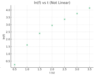
Not linear, therefore not exponential. Try $\ln(f)$ vs. $t$ plot:
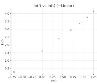
Not linear, therefore not exponential. Try $\ln(f)$ vs. $\ln(t)$ plot:
Approximately linear, therefore suggests a power series model. Linear regression on $\ln(f)$ vs. $\ln(t)$ using GDC: We get: $m = 1.966$ $ $ $ This is a power model. |
A semi-log graph is a type of graph that uses a logarithmic scale for one axis (usually the y-axis) and a linear scale for the other axis (usually the x-axis). A log-log graph, on the other hand, uses a logarithmic scale for both the x-axis and the y-axis.
Semi-log Graph
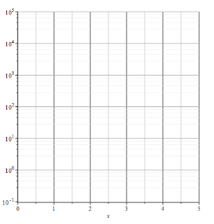
In a semi-log graph, the y-axis is scaled logarithmically, and the x-axis is scaled linearly. This means that each unit on the y-axis represents a tenfold increase in the value, while the x-axis increases by equal intervals.
Semi-log graphs are particularly useful when plotting data that spans several orders of magnitude or when the data follows an exponential trend. The most common example is exponential growth or decay, such as population growth, radioactive decay, or the spread of a virus.
For example, consider the exponential function:
$y = ab^x$
Taking the logarithm of both sides gives:
$\log(y) = \log(a) + x \log(b)$
This equation is linear in x, which means that when y is plotted on a logarithmic scale and x is plotted on a linear scale, the graph will be a straight line.
Log-log Graph
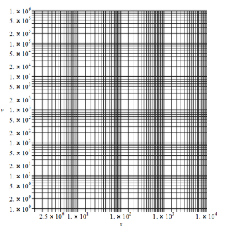
In a log-log graph, both the x-axis and the y-axis are scaled logarithmically. This type of graph is used when both variables cover a large range of values and when the relationship between the variables is a power law.
A power law has the form:
$y = ax^k$
Taking the logarithm of both sides gives:
$\log(y) = \log(a) + k \log(x)$
This is a linear equation in \(\log(x)\), meaning that if both axes are logarithmic, the graph will be a straight line. The slope of the line corresponds to the exponent \(k\), and the y-intercept corresponds to \(\log(a)\).
Log-log graphs are often used in physics, engineering, and other sciences to analyze relationships between variables that span many orders of magnitude.