Home / IB DP Maths 2026, 2027 & 2028 / Application and Interpretation HL / IBDP MAI : AHL 4.13 Non-linear regression

IB Mathematics AHL 4.13 Non-linear regression. AI HL Paper 3- Exam Style Questions- New Syllabus

Question

An investigation is carried out to contrast the final results of two different educational institutions, School $A$ and School $B$.
Every student at both institutions sits the same concluding examination at age $18$. A researcher named Aayush is evaluating these outcomes.
Aayush selects a representative group of $6$ students from each institution to participate in detailed interviews regarding their performance.
(a) (i) Identify one benefit of utilizing a larger sample size for this study.
(ii) Identify one drawback of increasing the number of students in the sample.
The percentages achieved by the $6$ sampled students from School $A$ are presented in Table $1$ below.
The average score for the School $A$ group is $51.7$ when rounded to $3$ significant figures.
(b) Calculate the value of the unbiased estimate of the population standard deviation, $s_{n-1}$, for the School $A$ sample.
The corresponding $s_{n-1}$ value for the School $B$ group is recorded as $7.66$.
Aayush suggests that: “The variation in marks at School $A$ is definitely lower than the variation at School $B$.”
(c) Provide one reason why Aayush’s conclusion might be flawed.
The exam authorities state that scores in both institutions follow an approximately normal distribution. Assume this information is valid.
Aayush intends to perform a pooled $t$-test to determine if there is a significant difference between the average marks of the two schools.
(d) (i) Specify the requirement regarding population variances that must be met to perform a pooled $t$-test. 
(ii) Determine if it is appropriate for Aayush to proceed with a pooled $t$-test here. Support your choice.
Before the study, Aayush hypothesized that School $B$ would have a higher average score than School $A$. His data shows that the average score for the School $B$ sample is exactly $60$.
(e) (i) Formulate the null and alternative hypotheses for this pooled $t$-test. 
(ii) Compute the $p$-value for the test. 
(iii) Using a $5\%$ significance level, state the conclusion of the test in the context of the study. Provide a justification. 
At age $11$, all students had previously taken the same entrance test.
Aayush wants to see if there is a relationship between the initial entrance test score and the final exam score. He obtains the age $11$ results for the $12$ students in his samples.
The Pearson’s product-moment correlation coefficient for these two sets of scores is $r = 0.876$. The critical value for $r$ at a $5\%$ significance level is $0.576$.
(f) (i) Conduct a hypothesis test at the $5\%$ level of significance. State your hypotheses and whether you reject the null hypothesis.
(ii) If the assumptions for a Pearson’s test are violated, name a more suitable correlation test to use.
The exam board uses a linear model to forecast a student’s final mark ($\hat{y}$) from their entrance mark ($x$): $\hat{y} = 0.37x + 37.6$
(g) Explain the contextual meaning of the gradient $0.37$ in this specific model.
Aayush calculates the “school value added” for each student using the formula $y – \hat{y}$ (rounded to $1$ decimal place). These values are shown in Table $2$.
(h) (i) Verify that the value represented by $q$ in Table $2$ is $0.6$.
(ii) Use a pooled $t$-test at the $5\%$ level to check if the average “school value added” is greater in School $A$ than in School $B$. State your hypotheses and justify your final decision. 
(i) Based on the various tests performed, explain how both School $A$ and School $B$ could each argue that they are the superior institution.

Most-appropriate topic codes (IB Mathematics Applications and Interpretation HL):

AHL 4.18: Hypothesis testing for population mean ($t$-tests) — parts (d), (e), (h)(ii) 
AHL 4.14: Unbiased estimates of population parameters ($s_{n-1}$) — parts (b), (c) 
AHL 4.13: Least squares regression analysis and predictions — part (g) 
SL 4.10: Spearman’s rank correlation coefficient — part (f)(ii) 
SL 4.4: Linear correlation and regression — part (f)(i)
SL 4.1: Concepts of sampling and reliability — part (a) 
▶️ Answer/Explanation

(a)(i)
Answer: The sample will be more reliable / more representative of the population / the sample mean is likely to be closer to the population mean. [cite: 1276]

(a)(ii)
Answer: More time consuming / expensive / more open to human error. [cite: 1411]

(b)
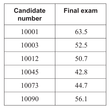
Method: Using GDC with data: $63.5, 52.5, 50.7, 42.8, 44.7, 56.1$
$\boxed{7.60}$ ($7.597537…$) [cite: 1431]

(c)
Answer: The population standard deviation may be different from the sample / these $s_{n-1}$ values are only estimates and the values are too close together / standard deviation is not the only measure of spread. [cite: 1431]

(d)(i)
Answer: The population variances are the same/equal. [cite: 1389]

(d)(ii)
Method: Compare sample standard deviations or variances
Sample $A$: $s_{n-1} = 7.60$, Sample $B$: $s_{n-1} = 7.66$
These are similar, so assumption of equal variances is plausible.
Yes, Aayush should use a pooled $t$-test. [cite: 1389]

(e)(i)
Answer: $H_0: \mu_A = \mu_B$, $H_1: \mu_A < \mu_B$ [cite: 1385]

(e)(ii)
Method: Using GDC with pooled $t$-test
Sample $A$: $n=6, \bar{x}=51.7, s=7.60$
Sample $B$: $n=6, \bar{x}=60, s=7.66$
$\boxed{0.0445}$ ($0.0444586…$) [cite: 1389]

(e)(iii)
Method: Compare $p$-value with significance level $\alpha = 0.05$
$0.0445 < 0.05$ $\Rightarrow$ Reject $H_0$
There is significant evidence that the population mean of School $B$ is higher than the population mean of School $A$ / Aayush’s belief is supported. [cite: 1385]

(f)(i)
Method: Correlation hypothesis test
$H_0: \rho = 0, H_1: \rho \neq 0$
Test statistic: $r = 0.876$
Critical value: $0.576$ (at $5\%$ significance level for $n=12$)
$0.876 > 0.576$ $\Rightarrow$ Reject $H_0$
There is significant evidence of correlation between entry exam and final exam results. [cite: 1465]

(f)(ii)
$\boxed{\text{Spearman’s rank correlation coefficient}}$ [cite: 1372]

(g)
As entry exam result increases by $1$ percentage point, the final exam result increases by $0.37$ percentage points.

(h)(i)
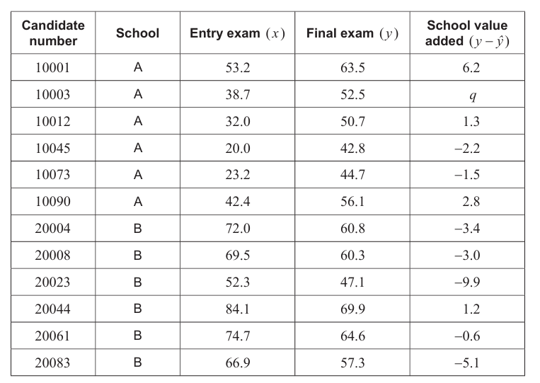
Method: For candidate $10003$: $x = 38.7$
Predicted: $\hat{y} = 0.37 \times 38.7 + 37.6 = 14.319 + 37.6 = 51.919$
School value added: $y – \hat{y} = 52.5 – 51.919 = 0.581$
Rounded to $1$ decimal place: $0.6$
$\boxed{0.6}$

(h)(ii)
Method: Pooled $t$-test on school value added data
$H_0: \mu_A = \mu_B$ (mean school value added equal)
$H_1: \mu_A > \mu_B$ (mean school value added higher in School $A$)
Using GDC with pooled $t$-test:
$p$-value $= 0.0213$ ($0.0212715…$)
$0.0213 < 0.05$ $\Rightarrow$ Reject $H_0$
There is evidence of higher school value added in School $A$. [cite: 1389, 1465]

(i)
Answer: School $B$ outperforms School $A$ is supported by the test in part (e) / higher mean. School $A$ outperforms School $B$ is supported by the test in part (h) / better added value.

Scroll to Top