
IBDP Physics SL Paper 1B- Data-Based Question- New Syllabus
Question
A student investigates whether the Stefan-Boltzmann law, \(L=4\pi\sigma R^{2}T^{4}\), applies to stars.
\(L=\) luminosity of the star, in W
\(\sigma=\) Stefan-Boltzmann constant
\(R=\) radius of the star, in m
\(T=\) surface temperature of the star, in K
To verify the law, they obtain values from databases and manipulate the data as shown.
| Star | \(L\) | \(R\) | \(T\) | \(\dfrac{L}{R^{2}}\) | \(\log\left(\dfrac{L}{R^{2}}\right)\) | \(\log(T)\) |
|---|---|---|---|---|---|---|
| 10 Lacertae | \(3.92\times10^{31}\) | \(5.75\times10^{9}\) | \(3.62\times10^{4}\) | \(1.19\times10^{12}\) | 12.1 | 4.56 |
| \(\sigma\)-Orionis A | \(1.60\times10^{31}\) | \(3.90\times10^{9}\) | \(3.49\times10^{4}\) | \(1.05\times10^{12}\) | 12.0 | 4.54 |
| \(\sigma\)-Orionis B | \(6.08\times10^{30}\) | \(3.48\times10^{9}\) | \(2.91\times10^{4}\) | \(5.02\times10^{11}\) | 11.7 | 4.46 |
| Polaris B | \(1.50\times10^{27}\) | \(9.60\times10^{8}\) | \(6.90\times10^{3}\) | \(1.63\times10^{9}\) | 9.21 | 3.84 |
| \(\alpha\)-Centauri A | \(5.77\times10^{26}\) | \(8.49\times10^{8}\) | \(5.79\times10^{3}\) | \(8.00\times10^{8}\) | 8.90 | 3.76 |
| \(\alpha\)-Centauri B | \(1.92\times10^{26}\) | \(5.97\times10^{8}\) | \(5.26\times10^{3}\) | \(5.39\times10^{8}\) | 8.73 | 3.72 |
| \(\epsilon\)-Indi | \(8.08\times10^{25}\) | \(4.95\times10^{8}\) | \(4.65\times10^{3}\) | \(3.30\times10^{8}\) | 8.52 | 3.67 |
| Sun | \(3.85\times10^{26}\) | \(6.96\times10^{8}\) | \(5.78\times10^{3}\) | \(7.95\times10^{8}\) | 8.90 | 3.76 |
(a) Complete the table with the missing values for Polaris B.
\(\boxed{\hspace{6cm}}\)
The student plots the variation in \(\log(T)\) of \(\log\left(\dfrac{L}{R^{2}}\right)\) and draws the line of best fit.
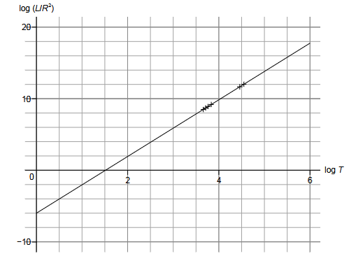
The student uses a GDC (graphical display calculator) to determine the equation of the line of best fit as
\(y=3.99x-6.15\)
(b) Explain how the gradient of the line of best fit relates to the Stefan-Boltzmann law.
\(\boxed{\hspace{9cm}}\)
(c) Calculate the Stefan-Boltzmann constant obtained in this investigation.
\(\boxed{\hspace{8cm}}\)
(d) Outline a conclusion for the investigation.
\(\boxed{\hspace{9cm}}\)
(e) Suggest a possible improvement of the investigation, related to the range of the surface temperatures of the stars selected.
\(\boxed{\hspace{9cm}}\)
▶️ Answer/Explanation
(a) Correct Answer: \( \boxed{1.63\times10^{9}} \) and \( \boxed{3.84} \)
For Polaris B,
\(\dfrac{L}{R^{2}}=\dfrac{1.50\times10^{27}}{(9.60\times10^{8})^{2}}\)
\(\dfrac{L}{R^{2}}\approx1.63\times10^{9}\)
Therefore,
\(\log\left(\dfrac{L}{R^{2}}\right)=\log(1.63\times10^{9})\approx9.21\)
Also, \(\log(6.90\times10^{3})\approx\boxed{3.84}\).
(b) Correct Answer:
The Stefan-Boltzmann law is
\(L=4\pi\sigma R^{2}T^{4}\)
Rearranging,
\(\dfrac{L}{R^{2}}=4\pi\sigma T^{4}\)
Taking logarithms gives
\(\log\left(\dfrac{L}{R^{2}}\right)=\log(4\pi\sigma)+4\log(T)\)
Comparing this with \(y=mx+c\), the gradient should therefore be \(4\).
The experimental gradient is \(3.99\), which is very close to \(4\), supporting the Stefan-Boltzmann law.
(c) Correct Answer: \( \boxed{5.63\times10^{-8}\,\mathrm{W\,m^{-2}\,K^{-4}}} \)
The intercept of the graph is \(-6.15\). From
\(\log\left(\dfrac{L}{R^{2}}\right)=4\log(T)+\log(4\pi\sigma)\)
the intercept is
\(\log(4\pi\sigma)=-6.15\)
Therefore,
\(4\pi\sigma=10^{-6.15}\)
\(\sigma=\dfrac{10^{-6.15}}{4\pi}\)
\(\sigma\approx5.63\times10^{-8}\,\mathrm{W\,m^{-2}\,K^{-4}}\)
Hence, \( \boxed{\sigma=5.63\times10^{-8}\,\mathrm{W\,m^{-2}\,K^{-4}}} \).
(d) Correct Answer:
The approximately linear graph has a gradient close to \(4\), as predicted by the Stefan-Boltzmann law.
The value of \(\sigma\) obtained experimentally is also close to the accepted value.
Therefore, the investigation provides evidence that the Stefan-Boltzmann law applies to stars.
(e) Correct Answer:
Use a wider range of stellar surface temperatures, including stars with temperatures both lower and higher than those currently selected. This would provide a greater range of data and make the relationship easier to test.