Forces and Their Effects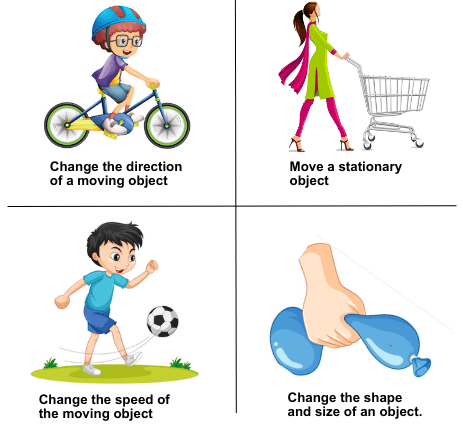
Forces can cause objects to undergo different changes. A force is a push or a pull acting on an object. When applied, it may produce changes in:
- Size: A force can stretch, compress, or deform an object (e.g., stretching a spring, squashing a sponge).
- Shape: A force can change the shape permanently or temporarily (e.g., bending a metal strip, molding clay).
- Motion: A force can make an object start moving, stop moving, speed up, slow down, or change direction (Newton’s laws of motion).
Example:
A football is at rest on the ground. When a player kicks it, the applied force changes its state of motion by making it move forward. If the player kicks harder, the ball also deforms slightly (change of shape) before regaining its round shape.
Resultant Force in a Straight Line
When two or more forces act along the same straight line (collinear forces), the resultant force is found by simple addition or subtraction:
- If the forces act in the same direction: \( F_\text{resultant} = F_1 + F_2 + \dots \)
- If the forces act in opposite directions: \( F_\text{resultant} = |F_\text{larger} – F_\text{smaller}| \)
- The direction of the resultant is the direction of the larger force.
Example:
Two people pull a box along the same line. One applies a force of \( 60~\text{N} \) to the right, and the other applies a force of \( 40~\text{N} \) to the left.
▶️ Answer/Explanation
Since the forces act in opposite directions: \( F_\text{resultant} = |60 – 40| = 20~\text{N} \).
The resultant force is \( 20~\text{N} \) to the right (direction of the larger force).
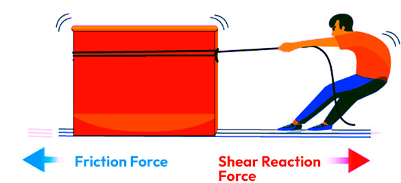
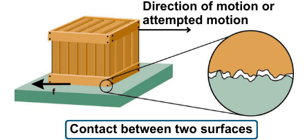
Friction
Friction is the force that opposes relative motion or the tendency of motion between two surfaces in contact. It always acts in the direction opposite to motion (or attempted motion). Friction is caused by the microscopic irregularities of surfaces and intermolecular forces between them.
Types of Friction:
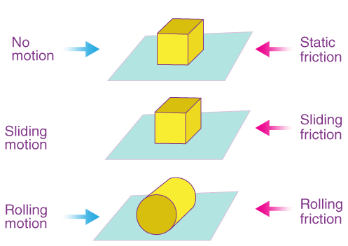
- Static friction: Acts when an object is at rest. It prevents motion until a maximum limit is reached. Example: A book stays on a tilted table until the tilt becomes too steep.
- Kinetic (sliding) friction: Acts when objects slide over each other. Example: Sliding a box across the floor.
- Rolling friction: Occurs when an object rolls over a surface, and is usually much smaller. Example: A car tire rolling on the road.
Effects of Friction:
- Impeding motion: Friction resists movement, so more force is needed to move objects.
- Heating: Friction converts kinetic energy into thermal energy, producing heat.
- Wear and tear: Continuous friction damages surfaces over time.
Advantages of Friction:
- Allows us to walk without slipping.
- Helps cars to grip the road, especially during turning or braking.
- Enables nails, screws, and bolts to stay fixed in place.
Disadvantages of Friction:
- Wastes energy as heat in engines and machinery.
- Causes wearing out of tyres, shoe soles, and machine parts.
- Makes moving heavy objects difficult.
Example
A wooden box of weight \( 100~\text{N} \) is placed on a horizontal floor. The maximum static friction force between the box and the floor is \( 40~\text{N} \).
▶️Answer/Explanation
Explanation:
- If a horizontal force of less than \( 40~\text{N} \) is applied, the box will not move because static friction balances it.
- If a horizontal force equal to or greater than \( 40~\text{N} \) is applied, the box will start moving. Once moving, kinetic friction (usually slightly less than static friction) will oppose the motion.
- As the box slides, friction produces heat at the contact surface.
Therefore: Friction first prevents motion, then resists it, while also converting some energy into heat.
Friction (Drag) in Liquids
When an object moves through a liquid (or even a gas like air), it experiences a resistive force called drag. This drag force is the liquid’s version of friction, acting opposite to the direction of motion.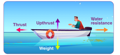
Key Points:
- Cause of drag: Drag arises because liquid particles collide with the surface of the moving object, creating resistance.
- Direction: Drag always acts opposite to motion.
- Dependence: The size of drag depends on:
- The speed of the object (faster speed = greater drag).
- The shape of the object (streamlined shapes reduce drag).
- The viscosity (thickness) of the liquid (thicker liquid = more drag).
- The surface area of the object in contact with the fluid.
- At high speeds, drag can become very significant, often balancing the driving force, leading to a constant speed called terminal velocity.
Everyday Examples:
- A swimmer feels water resistance (drag) as they push forward.
- A ship moving through water experiences drag, requiring powerful engines to keep moving.
- A stone dropped into water slows down due to drag until it sinks steadily.
Example :
A small ball is dropped into a liquid. At first, it accelerates due to gravity, but soon the upward drag force increases. Finally, the drag force equals the weight of the ball.
▶️Answer/Explanation
Explanation:
- Initially: Acceleration is maximum as only weight acts significantly.
- As speed increases: Drag increases, reducing net acceleration.
- Finally: Drag = Weight ⟹ Net force = 0, so the ball falls at a constant speed (terminal velocity).
Friction (Drag) in Gases – Air Resistance:
When an object moves through a gas such as air, it experiences a resistive force called air resistance (a type of drag). This force always acts opposite to the direction of motion, reducing the object’s speed.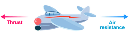
- Cause: Air particles collide with the surface of the moving object, creating resistance.
- Direction: Always opposite to the object’s motion.
Factors affecting air resistance:
- Speed of object: Faster objects experience greater air resistance.
- Surface area: A larger surface area facing motion increases air resistance (e.g., parachute).
- Shape of object: Streamlined shapes reduce drag, while irregular shapes increase it.
- Density of air: Thicker air (humid or at lower altitudes) increases drag.
Example:
A skydiver jumps out of an aircraft and falls through the air.
▶️Answer/Explanation
At first: Air resistance is small, so the skydiver accelerates downward due to gravity.
As speed increases: Air resistance builds up, opposing motion more strongly.
Eventually: Air resistance balances weight. Resultant force = 0. The skydiver reaches terminal velocity (constant speed).
With parachute: Surface area increases drastically, drag becomes much larger, reducing the skydiver’s speed to a safe landing velocity.
Newton’s First Law of Motion:
An object will remain at rest, or continue to move in a straight line at constant speed, unless acted upon by a resultant force.
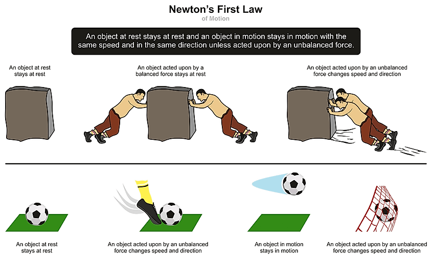
- If resultant force = 0:
- An object at rest stays at rest.
- An object in motion keeps moving in the same direction at the same speed (constant velocity).
- If resultant force ≠ 0:
- The object’s state of motion changes (it may accelerate, decelerate, or change direction).
Example:
A book lying on a table will remain at rest unless you apply a force to move it.
▶️Answer/Explanation
- At rest: No resultant force acts on the book (forces are balanced: weight down, table’s support up).
- In motion: If you slide the book, friction acts as a resultant force opposing motion, so the book eventually stops.
- Conclusion: Without a resultant force, the object would continue to move in a straight line at constant speed (ideal case with no friction).
Newton’s Second Law
Newton’s Second Law can also be stated as:
“The resultant force acting on an object is equal to the rate of change of its momentum.”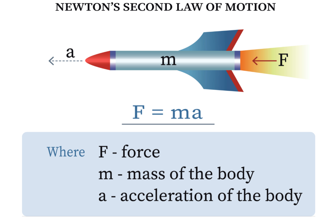
Mathematically:
\( F = \dfrac{\Delta p}{\Delta t} \)
- \( p \) = momentum = \( mv \)
- \( \Delta p \) = change in momentum
- \( \Delta t \) = time taken for the change
Derivation of \( F = ma \):
- Momentum of an object is given by \( p = mv \).
- The rate of change of momentum:
- \( F = \dfrac{\Delta p}{\Delta t} = \dfrac{\Delta (mv)}{\Delta t} \)
- If the mass \( m \) is constant:
- \( F = m \dfrac{\Delta v}{\Delta t} \)
- But \( \dfrac{\Delta v}{\Delta t} = a \), the acceleration.
- So: \( F = ma \)
Therefore, Newton’s Second Law can be expressed in two equivalent ways:
- \( F = \dfrac{\Delta p}{\Delta t} \) → General form (for changing momentum)
- \( F = ma \) → Special case (when mass is constant)
Example:
A ball of mass \( 2~\text{kg} \) changes its velocity from \( 4~\text{m/s} \) to \( 10~\text{m/s} \) in \( 3~\text{s} \). Find the resultant force on the ball.
▶️Answer/Explanation
Momentum change: \( \Delta p = m \Delta v = 2(10 – 4) = 12~\text{kg m/s} \).
Time taken = 3 s.
Force: \( F = \dfrac{\Delta p}{\Delta t} = \dfrac{12}{3} = 4~\text{N} \).
The force acting on the ball is \( 4~\text{N} \).
Load–Extension Graphs for an Elastic Solid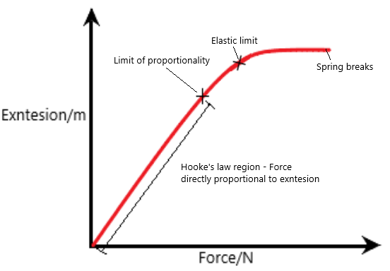
Definitions
- Load = the force applied to the object (usually measured in newtons, N).
- Extension = the increase in length produced by the load (measured in metres, m or mm).
- For an elastic solid that obeys Hooke’s law over some range: the load is proportional to the extension.
Hooke’s law (linear region)
Within the proportional limit: \( F \propto x \) so \( F = k x \), where \( k \) is the spring (force) constant in \( \text{N/m} \).
Apparatus (typical)
- A clamp stand with boss and clamp
- A spring or wire (test specimen)
- Set of small masses and hanger (or calibrated force sensor)
- Meter rule (or vernier gauge) to measure length/extension
- Pointer attached to spring end (optional, improves reading)
- Graph paper or computer plotting software
Experimental Procedure (step-by-step)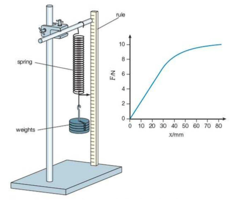
- Secure the spring (or wire) vertically with one end fixed in the clamp; hang a pointer from the free end aligned with a scale for accurate reading.
- Measure and record the natural (unstretched) length \( L_0 \) of the spring.
- Add a small known load (mass on hanger). Wait until the spring settles and measure the new length \( L \). Calculate extension \( x = L – L_0 \).
- Record the load as the weight: \( F = mg \) (use \( g = 9.8~\text{N/kg} \) unless instructed otherwise). If using a force sensor, read force directly.
- Repeat for several increasing loads (add masses stepwise). Take at least 6–8 readings covering small to larger extensions, but do not exceed the elastic limit (do not permanently deform the spring).
- For accuracy, repeat each reading a few times and take the mean extension for each load. Remove and rehang the masses to check repeatability.
- Plot the graph: vertical axis (y) = Load \( F \) (N); horizontal axis (x) = Extension \( x \) (m or mm). Label axes with units.
- Draw the best-fit line through the points in the initial linear region. Determine slope \( \dfrac{\Delta F}{\Delta x} \) — this slope equals the spring constant \( k \).
- Optional: remove loads gradually and plot unloading points. If unloading path coincides with loading, behaviour is perfectly elastic; if not, hysteresis indicates energy loss (e.g. internal friction).
How to sketch / what to expect on the plot
- Linear region (Hooke’s law): The initial portion is a straight line through the origin (or near origin) — here \( F = kx \).
- Limit of proportionality: The point beyond which the graph ceases to be a straight line — proportionality breaks down.
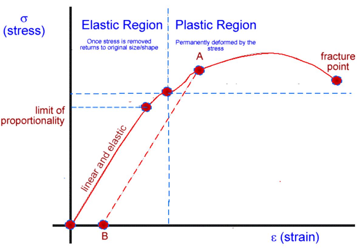
- Elastic limit: The maximum load beyond which the solid will not return to original length (permanent deformation). If you exceed this, on unloading the object will not return to \( L_0 \).
- Plastic region: If the specimen is stretched beyond elastic limit it enters a plastic region (curve does not return on unloading).
- Breaking point (if tested to failure): The graph may show a maximum load where the specimen breaks.
- Area under graph (in linear region): equals the elastic potential energy stored: \( E = \tfrac{1}{2} F x = \tfrac{1}{2} k x^2 \) (work done to stretch from 0 to \( x \)).
Interpretation (how to read the graph)
- Slope: \( \text{slope} = \dfrac{\Delta F}{\Delta x} = k \). A steep slope ⇒ stiff spring (large \( k \)).
- Straight line through origin: Hookean behaviour (proportionality). If the line does not pass exactly through origin, consider small systematic errors (zero-offset) and correct readings.
- Deviation from linearity: Indicates limit of proportionality or onset of plastic behaviour.
- Hysteresis (loading vs unloading loop): Area of loop = energy dissipated as heat/internal friction during cycle.
Precautions & sources of error
- Use small incremental loads to remain within elastic region.
- Allow readings to settle (wait for oscillations to die out).
- Measure extension from the same reference point each time; use a pointer to reduce parallax.
- Temperature changes may affect material behaviour; perform experiment at constant temperature if possible.
- Account for the mass of the hanger and pointer when computing total load.
- Take several readings and average to reduce random error.
Example
A spring has natural length \( L_0 = 0.120~\text{m} \). The following data were recorded:
- Mass added \( 0.05~\text{kg} \) → length \( 0.140~\text{m} \)
- Mass added \( 0.10~\text{kg} \) → length \( 0.160~\text{m} \)
- Mass added \( 0.15~\text{kg} \) → length \( 0.179~\text{m} \)
Use \( g = 9.8~\text{N/kg} \). Determine
(a) the extensions,
(b) the forces (loads),
(c) estimate the spring constant \( k \) from the slope using the first two points, and
(d) the elastic potential energy stored when the mass is \( 0.15~\text{kg} \).
▶️Answer/Explanation
Step (a) – Extensions:
For \( 0.05~\text{kg} \): extension \( x_1 = 0.140 – 0.120 = 0.020~\text{m} \).
For \( 0.10~\text{kg} \): extension \( x_2 = 0.160 – 0.120 = 0.040~\text{m} \).
For \( 0.15~\text{kg} \): extension \( x_3 = 0.179 – 0.120 = 0.059~\text{m} \).
Step (b) – Loads (weights):
\( F_1 = 0.05 \times 9.8 = 0.49~\text{N} \)
\( F_2 = 0.10 \times 9.8 = 0.98~\text{N} \)
\( F_3 = 0.15 \times 9.8 = 1.47~\text{N} \)
Step (c) – Estimate spring constant \( k \) from first two points (slope):
Slope \( k \approx \dfrac{\Delta F}{\Delta x} = \dfrac{F_2 – F_1}{x_2 – x_1} = \dfrac{0.98 – 0.49}{0.040 – 0.020} = \dfrac{0.49}{0.020} = 24.5~\text{N/m} \).
Step (d) – Elastic potential energy at \( 0.15~\text{kg} \):
Use \( E = \tfrac{1}{2} k x^2 \). Using \( k = 24.5~\text{N/m} \) (estimate) and \( x_3 = 0.059~\text{m} \):
\( E = \tfrac{1}{2} \times 24.5 \times (0.059)^2 \approx 0.5 \times 24.5 \times 0.003481 = 0.0426~\text{J} \) (≈ \(4.3 \times 10^{-2}~\text{J}\)).
Notes: If you plot all three points and draw a best-fit straight line through the linear region, you would get a slightly more accurate \( k \). The small discrepancy in the third point (0.059 vs exact 0.060) may indicate either slight nonlinearity or reading uncertainty.
Spring Constant
The spring constant (denoted by \( k \)) is defined as the force required to produce unit extension in a spring or elastic object. In other words, it measures the stiffness of the spring. A large value of \( k \) means the spring is very stiff and requires more force to stretch by the same amount.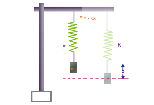
Equation:
$ k = \frac{F}{x} $
where:
- \( k \) = spring constant (N/m)
- \( F \) = applied force (N)
- \( x \) = extension produced (m)
Hooke’s Law form:
$ F = kx $
Interpretation:
- The slope of a load–extension graph in the linear (Hookean) region gives the spring constant.
- A stiffer spring → steeper slope → larger \( k \).
Example:
A spring extends by \( 0.04~\text{m} \) when a load of \( 2.0~\text{N} \) is applied. Calculate the spring constant.
▶️Answer/Explanation
We know: $ k = \frac{F}{x} $
Substitute values: $ k = \frac{2.0}{0.04} = 50~\text{N/m} $
Final Answer: The spring constant is \( 50~\text{N/m} \).
Limit of Proportionality
The limit of proportionality is the point on a load–extension graph beyond which the extension of a material is no longer directly proportional to the applied load. In simpler terms, the spring or wire stops obeying Hooke’s law beyond this point.
On a graph:
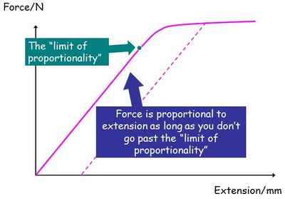
- Before the limit of proportionality → straight line (linear region) → \( F \propto x \) → \( F = kx \)
- Beyond the limit of proportionality → curve begins → force is no longer proportional to extension
Key Points:
- The limit of proportionality is usually slightly less than the elastic limit (but detailed elastic limit knowledge is not required).
- It is the maximum load for which Hooke’s law is valid.
- Identifying it on a graph: the point where the straight line first starts to curve.
Example:
A spring is tested with increasing loads. The load–extension graph is linear up to a load of \( 5~\text{N} \), after which the graph starts to curve. Identify the limit of proportionality.
▶️Answer/Explanation
The graph remains straight (linear) up to \( 5~\text{N} \). Beyond this, it starts to curve.
Therefore, the limit of proportionality is \( 5~\text{N} \).