Graphs of Functions
1. Construct Tables of Values and Draw Graphs
To draw graphs of functions, follow these steps:
- Choose a set of x-values (e.g., from –3 to 3).
- Substitute into the function to calculate y-values.
- Complete a table of values.
- Plot the coordinates (x, y) on a grid.
- Join the points smoothly if needed (especially for curves).
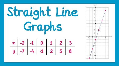
Graph Type 1: Linear Function – \( y = ax + b \)
These graphs are straight lines. The coefficient \( a \) is the gradient and \( b \) is the y-intercept.
Example:
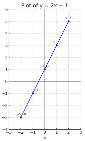
Draw the graph of \( y = 2x + 1 \) for \( x = -2 \) to \( 2 \).
▶️ Answer/Explanation
Table of values:
| x | –2 | –1 | 0 | 1 | 2 |
|---|---|---|---|---|---|
| y = 2x + 1 | –3 | –1 | 1 | 3 | 5 |
Plot and join points with a straight line.
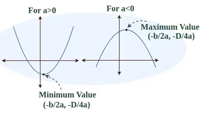
Graph Type 2: Quadratic Function – \( y = \pm x^2 + ax + b \)
These graphs form U-shaped curves (parabolas). If the coefficient of \( x^2 \) is positive, the graph opens upwards; if negative, it opens downwards.
Example:
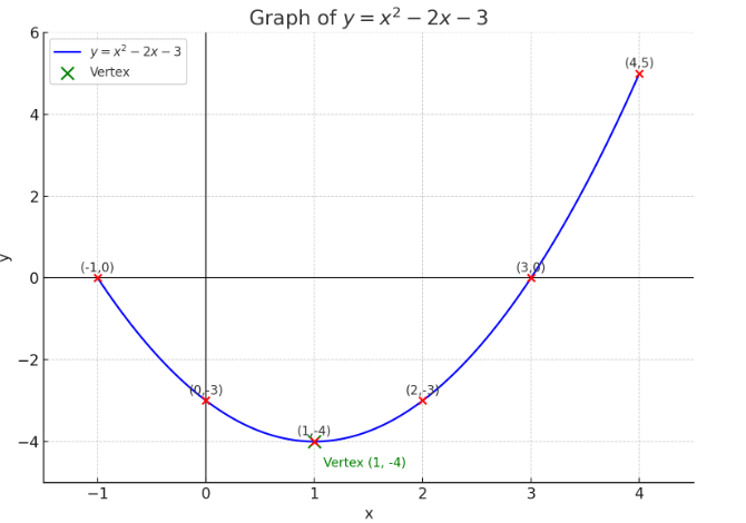
Draw the graph of \( y = x^2 – 2x – 3 \) for \( x = -1 \) to \( 4 \).
▶️ Answer/Explanation
Table of values:
| x | –1 | 0 | 1 | 2 | 3 | 4 |
|---|---|---|---|---|---|---|
| y = x² – 2x – 3 | 0 | –3 | –4 | –3 | 0 | 5 |
Plot the points and join with a smooth curve.
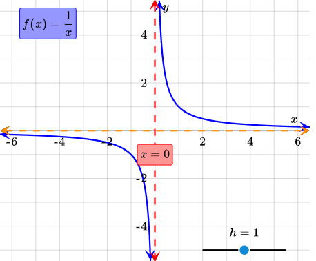
Graph Type 3: Reciprocal Function – \( y = \frac{x}{a} \text{ or } \frac{1}{x} \)
These are not straight lines. They form curves with asymptotes (lines the graph approaches but never touches). For example, \( y = \frac{1}{x} \) is undefined at \( x = 0 \).
Example:
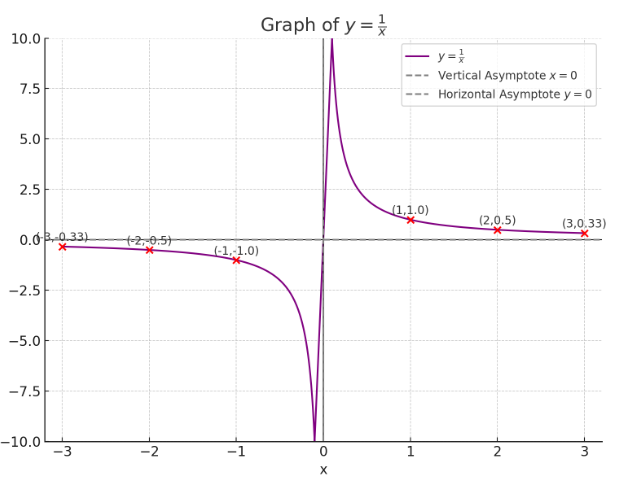
Draw the graph of \( y = \frac{1}{x} \) for \( x = -3 \) to \( 3 \), excluding 0.
▶️ Answer/Explanation
Table of values:
| x | –3 | –2 | –1 | 1 | 2 | 3 |
|---|---|---|---|---|---|---|
| y = 1/x | –0.333 | –0.5 | –1 | 1 | 0.5 | 0.333 |
Plot the points carefully and sketch two smooth branches — one in each quadrant. Note: The graph never touches the x or y axes.
Tips for Drawing and Interpreting Graphs:
- Use a ruler for straight-line graphs and smooth curves for quadratics and reciprocals.
- Always label axes and scales clearly.
- Indicate turning points and asymptotes if applicable.
- Use symmetry in quadratic and reciprocal graphs where appropriate.
Graphs of Algebraic and Exponential Functions
- Polynomial graphs: of the form \( ax^n \), where \( n = 1, 2, 3 \)
- Exponential graphs: of the form \( ab^x + c \)
Steps to Draw a Graph:
- Choose a range of \( x \)-values (e.g., from –3 to 3).
- Substitute into the function to find corresponding \( y \)-values.
- Plot the points on a coordinate grid.
- Join the points with a smooth curve or straight line.
Example:
Draw the graph of \( y = 2x + 1 \) for \( -3 \leq x \leq 3 \)
▶️ Answer/Explanation
Construct a table of values:
\( \begin{array}{c|c} x & y = 2x + 1 \\ \hline -3 & -5 \\ -2 & -3 \\ -1 & -1 \\ 0 & 1 \\ 1 & 3 \\ 2 & 5 \\ 3 & 7 \\ \end{array} \)
Plot and join the points to form a straight line.
Example :
Draw the graph of \( y = x^2 – 2x \) for \( -1 \leq x \leq 4 \)
▶️ Answer/Explanation
\( \begin{array}{c|c} x & y = x^2 – 2x \\ \hline -1 & 3 \\ 0 & 0 \\ 1 & -1 \\ 2 & 0 \\ 3 & 3 \\ 4 & 8 \\ \end{array} \)
This is a parabola opening upwards. Plot the points and draw a smooth curve.
Example :
Draw the graph of \( y = x^3 – x \) for \( -2 \leq x \leq 2 \)
▶️ Answer/Explanation
\( \begin{array}{c|c} x & y = x^3 – x \\ \hline -2 & -6 \\ -1 & 0 \\ 0 & 0 \\ 1 & 0 \\ 2 & 6 \\ \end{array} \)
This is a cubic curve with turning points. Plot and draw a smooth S-shaped curve.
Example :
Draw the graph of \( y = 2^x + 1 \) for \( -2 \leq x \leq 3 \)
▶️ Answer/Explanation
\( \begin{array}{c|c} x & y = 2^x + 1 \\ \hline -2 & 1.25 \\ -1 & 1.5 \\ 0 & 2 \\ 1 & 3 \\ 2 & 5 \\ 3 & 9 \\ \end{array} \)
This is an exponential growth curve. The graph gets steeper as \( x \) increases.
Solving Equations Graphically
Graphical methods allow us to solve equations by plotting them and visually identifying the solution(s). This is particularly useful for equations that are difficult or impossible to solve algebraically (such as non-linear equations or simultaneous equations involving curves).
What It Means to Solve Graphically:
- Solving equations: To solve \( f(x) = g(x) \), we graph both functions \( y = f(x) \) and \( y = g(x) \). The x-values at which the graphs intersect are the solutions.
- Finding roots of a function: The solutions to \( f(x) = 0 \) are where the graph of \( y = f(x) \) crosses the x-axis.
- Solving inequalities: You can also use graphs to identify intervals where one graph lies above or below another (for \( f(x) > g(x) \), etc.).
When to Use Graphical Methods:
- When solving equations involving linear vs. curve (e.g. \( x + 3 = x^2 \))
- To check or estimate the number of real solutions visually
- When given tables of values or required to construct your own
Steps to Solve an Equation Graphically:
- Rewrite the equation as two separate expressions (e.g., for \( x^2 + 2x = x + 6 \), write: \( y = x^2 + 2x \) and \( y = x + 6 \)).
- Create tables of values for both expressions.
- Plot both graphs on the same set of axes, using the same scale.
- Find the point(s) where the graphs intersect — the x-values of these points are the solutions.
Example:
Solve graphically: \( x^2 + 2x = x + 6 \)
▶️ Answer/Explanation
Step 1: Rewrite as two equations:
- \( y = x^2 + 2x \)
- \( y = x + 6 \)
Step 2: Plot both graphs for a range of \( x \) (e.g. from –4 to 2)
Table for \( y = x^2 + 2x \):
| x | –4 | –3 | –2 | –1 | 0 | 1 |
|---|---|---|---|---|---|---|
| y | 8 | 3 | 2 | –1 | 0 | 3 |
Table for \( y = x + 6 \):
| x | –4 | –3 | –2 | –1 | 0 | 1 |
|---|---|---|---|---|---|---|
| y | 2 | 3 | 4 | 5 | 6 | 7 |
Step 3: Plot the two graphs and find their intersection points.
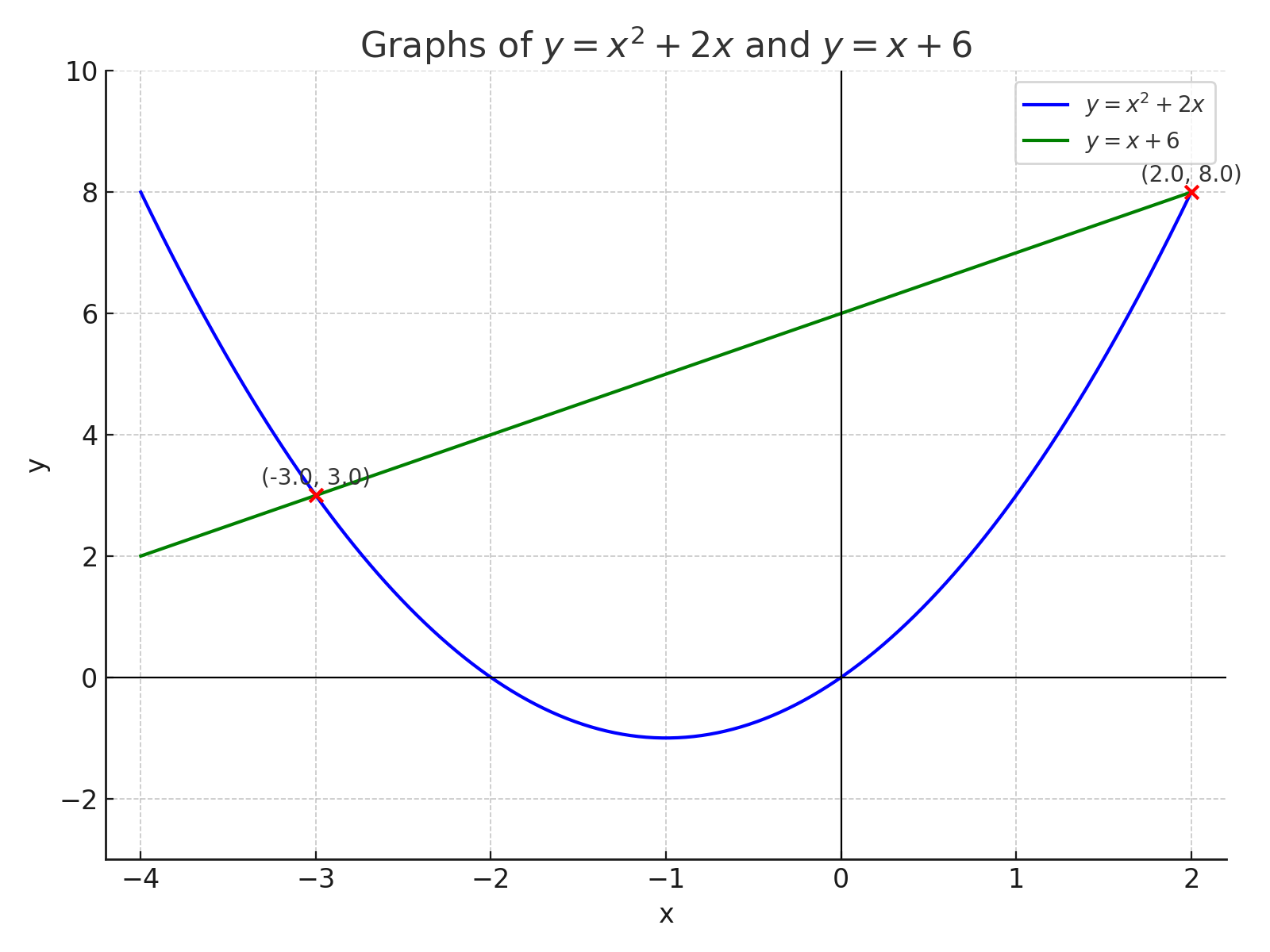
The curves intersect at \( x = –3 \) and \( x = -2 \)
Answer: The solutions are \( x = –3 \) and \( x =- 2 \)
Note:
- Always label both graphs and clearly show the points of intersection.
- Roots of a function are the x-values where the graph intersects the x-axis (i.e., where \( y = 0 \)).
- Use graphing software or a GDC for accuracy in exams if allowed.
Exponential Growth and Decay: Graphs
Exponential growth and decay are real-life processes where quantities increase or decrease rapidly over time. These can be modelled using exponential functions and represented using graphs.
General Form of an Exponential Function:
\( y = ab^x + c \), where:
- \( a \): Initial value
- \( b \): Growth/decay factor (if \( b > 1 \), it’s growth; if \( 0 < b < 1 \), it’s decay)
- \( x \): Time or input variable
- \( c \): Vertical shift (can be 0 in many models)
Key Features of the Graph:
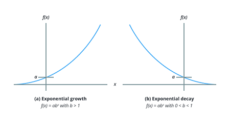
- Curved graph, not a straight line
- For growth, the graph increases rapidly
- For decay, the graph decreases and approaches zero (asymptote)
- Always positive if the model represents quantities like population or money
Example :
A population of bacteria doubles every hour. Initially, there are 50 bacteria. Represent this using a graph for 0 to 5 hours.
▶️ Answer/Explanation
Let \( y = 50 \cdot 2^x \), where \( x \) is time in hours.
\( \begin{array}{c|c} x (\text{hours}) & y = 50 \cdot 2^x \\ \hline 0 & 50 \\ 1 & 100 \\ 2 & 200 \\ 3 & 400 \\ 4 & 800 \\ 5 & 1600 \\ \end{array} \)
The graph is a steep curve rising rapidly. It shows exponential growth.
Example :
A car loses 20% of its value each year. It costs $\$20,000$ now. Represent the value over the next 5 years.
▶️ Answer/Explanation
Each year, the value is multiplied by 0.8 (since $20\%$ is lost).
Let \( y = 20000 \cdot (0.8)^x \), where \( x \) is years.
\( \begin{array}{c|c} x (\text{years}) & y = 20000 \cdot (0.8)^x \\ \hline 0 & 20000 \\ 1 & 16000 \\ 2 & 12800 \\ 3 & 10240 \\ 4 & 8192 \\ 5 & 6553.6 \\ \end{array} \)
The graph is a downward curve that gets flatter, showing exponential decay.
Example :
A population is modeled by \( y = 500 \cdot 1.05^x – 30 \). Plot this for \( 0 \leq x \leq 5 \).
▶️ Answer/Explanation
\( \begin{array}{c|c} x & y = 500 \cdot 1.05^x – 30 \\ \hline 0 & 470 \\ 1 & 464.5 \\ 2 & 486.73 \\ 3 & 510.07 \\ 4 & 534.57 \\ 5 & 560.3 \\ \end{array} \)
This is still exponential growth but shifted downward initially due to –30.