Question
The figure below shows the lengths in centimetres of fish found in the net of a small trawler.
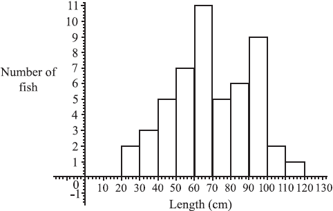
Find the total number of fish in the net.[2]
Find (i) the modal length interval,
(ii) the interval containing the median length,
(iii) an estimate of the mean length.[5]
(i) Write down an estimate for the standard deviation of the lengths.
(ii) How many fish (if any) have length greater than three standard deviations above the mean?[3]
The fishing company must pay a fine if more than 10% of the catch have lengths less than 40cm.
Do a calculation to decide whether the company is fined.[2]
A sample of 15 of the fish was weighed. The weight, W was plotted against length, L as shown below.
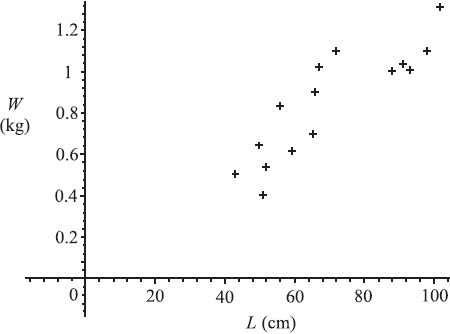
Exactly two of the following statements about the plot could be correct. Identify the two correct statements.
Note: You do not need to enter data in a GDC or to calculate r exactly.
(i) The value of r, the correlation coefficient, is approximately 0.871.
(ii) There is an exact linear relation between W and L.
(iii) The line of regression of W on L has equation W = 0.012L + 0.008 .
(iv) There is negative correlation between the length and weight.
(v) The value of r, the correlation coefficient, is approximately 0.998.
(vi) The line of regression of W on L has equation W = 63.5L + 16.5.[2]
Answer/Explanation
Markscheme
Total = 2 + 3 + 5 + 7 + 11 + 5 + 6 + 9 + 2 + 1 (M1)
(M1) is for a sum of frequencies.
= 51 (A1)(G2)[2 marks]
Unit penalty (UP) is applicable where indicated in the left hand column.
(i) modal interval is 60 – 70
Award (A0) for 65 (A1)
(ii) median is length of fish no. 26, (M1)(A1)
also 60 – 70 (G2)
Can award (A1)(ft) or (G2)(ft) for 65 if (A0) was awarded for 65 in part (i).
(iii) mean is \(\frac{{2 \times 25 + 3 \times 35 + 5 \times 45 + 7 \times 55 + …}}{{51}}\) (M1)
(UP) = 69.5 cm (3sf) (A1)(ft)(G1)
Note: (M1) is for a sum of (frequencies multiplied by midpoint values) divided by candidate’s answer from part (a). Accept mid-points 25.5, 35.5 etc or 24.5, 34.5 etc, leading to answers 70.0 or 69.0 (3sf) respectively. Answers of 69.0, 69.5 or 70.0 (3sf) with no working can be awarded (G1).[5 marks]
Unit penalty (UP) is applicable where indicated in the left hand column.
(UP) (i) standard deviation is 21.8 cm (G1)
For any other answer without working, award (G0). If working is present then (G0)(AP) is possible.
(ii) \(69.5 + 3 \times 21.8 = 134.9 > 120\) (M1)
no fish (A1)(ft)(G1)
For ‘no fish’ without working, award (G1) regardless of answer to (c)(i). Follow through from (c)(i) only if method is shown.[3 marks]
5 fish are less than 40 cm in length, (M1)
Award (M1) for any of \(\frac{5}{51}\), \(\frac{46}{51}\), 0.098 or 9.8%, 0.902, 90.2% or 5.1 seen.
hence no fine. (A1)(ft)
Note: There is no G mark here and (M0)(A1) is never allowed. The follow-through is from answer in part (a).[2 marks]
(i) and (iii) are correct. (A1)(A1)[2 marks]
Question
The speed, \(s\) , in \({\text{km }}{{\text{h}}^{ – 1}}\), of \(120\) vehicles passing a point on the road was measured. The results are given below.
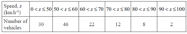
Write down the midpoint of the \(60 < s \leqslant 70\) interval.[1]
Use your graphic display calculator to find an estimate for
(i) the mean speed of the vehicles;
(ii) the standard deviation of the speeds of the vehicles.[3]
Write down the number of vehicles whose speed is less than or equal to \({\text{60 km }}{{\text{h}}^{ – 1}}\).[1]
Consider the cumulative frequency table below.
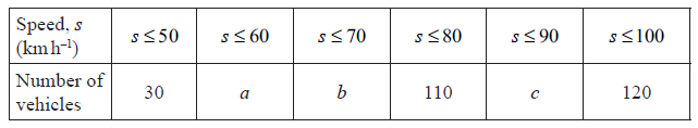
Write down the value of \(a\) , of \(b\) and of \(c\) .[2]
Consider the cumulative frequency table below.

Draw a cumulative frequency graph for the information from the table. Use \(1\) cm to represent \({\text{10 km }}{{\text{h}}^{ – 1}}\) on the horizontal axis and \(1\) cm to represent \(10\) vehicles on the vertical axis.[4]
Use your cumulative frequency graph to estimate
(i) the median speed of the vehicles;
(ii) the number of vehicles that are travelling at a speed less than or equal to \({\text{65 km }}{{\text{h}}^{ – 1}}\).[4]
All drivers whose vehicle’s speed is greater than one standard deviation above the speed limit of \({\text{50 km }}{{\text{h}}^{ – 1}}\) will be fined.
Use your graph to estimate the number of drivers who will be fined.[3]
Answer/Explanation
Markscheme
\(65\) (A1)[1 mark]
(i) \(54{\text{ (km }}{{\text{h}}^{ – 1}})\) (G2)
Note: If the answer to part (b)(i) is consistent with the answer to part (a) then award (G2)(ft) even if no working seen.
(ii) \(19.2\) (\(19.2093 \ldots \)) (G1)
Note: Accept \(19\), do not accept \(20\).[3 marks]
\(76\) (A1)[1 mark]
\(a = 76\), \(b = 98\) (A1)(ft)
Note: Follow through from their answer to part (c) for \(a\) and \(b = \) their \(a + 22\) .\(c = 118\) (A1)
[2 marks]
 (A1)(A1)(ft)(A1)(ft)(A1)
Notes: Award (A1) for axes labelled and correct scales. If the axes are reversed do not award this mark but follow through. Award (A2)(ft) for their 6 points correct, (A1)(ft) for at least 3 of these points correct. Award (A1) for smooth curve drawn through all points including (\(0\), \(0\)). If either the \(x\) or the \(y\) axis has a break in it to zero, do not award this final mark.[4 marks]
(i) \(57\) \({\text{(km }}{{\text{h}}^{ – 1}})\) \(( \pm 2)\) (M1)(A1)(ft)(G2)
Note: Award (M1) for clear indication of median on their graph. Follow through from their graph. If their answer is consistent with their incorrect graph but there is no working present on graph then no marks are awarded.
(ii) \(90\) vehicles \(( \pm 2)\) (M1)(A1)(ft)(G2)
Note: Award (M1) for clear indication of method on their graph. Follow through from their graph. If their answer is consistent with their incorrect graph but there is no working present on graph then no marks are awarded.[4 marks]
\(50 + 19.2 = 69.2\) (A1)(ft)
\(24\) \(( \pm 2)\) drivers will be fined (M1)(A1)(ft)(G2)
Notes: Follow through from their graph and from their part (b)(ii). Award (M1) for indication of method on their graph. If their answer is consistent with their incorrect graph but there is no working present on graph then no marks are awarded.[3 marks]
Question
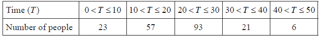
200 people were asked the amount of time T (minutes) they had spent in the supermarket. The results are represented in the table below.
State if the data is discrete or continuous.[1]
State the modal group.[1]
Write down the midpoint of the interval 10 < T ≤ 20 .[1]
Use your graphic display calculator to find an estimate for
(i) the mean;
(ii) the standard deviation.[3]
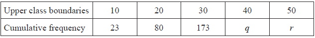
The results are represented in the cumulative frequency table below, with upper class boundaries of 10, 20, 30, 40, 50.
Write down the value of
(i) q;
(ii) r.[2]
The results are represented in the cumulative frequency table below, with upper class boundaries of 10, 20, 30, 40, 50.

On graph paper, draw a cumulative frequency graph, using a scale of 2 cm to represent 10 minutes (T) on the horizontal axis and 1 cm to represent 10 people on the vertical axis.[4]
Use your graph from part (f) to estimate
(i) the median;
(ii) the 90th percentile of the results;
(iii) the number of people who shopped at the supermarket for more than 15 minutes.[6]
Answer/Explanation
Markscheme
continuous (A1)[1 mark]
20 < T ≤ 30 (A1)[1 mark]
15 (A1)[1 mark]
(i) 21.5 (G2)
(ii) 9.21 (9.20597…) (G1)[3 marks]
(i) q = 194 (A1)
(ii) r = 200 (A1)[2 marks]
 (A1)(A2)(ft)(A1)
Notes: Award (A1) for scale and axis labels, (A2)(ft) for 5 correct points, (A1)(ft) for 4 or 3 correct points, (A0) for less than 3 correct points, (A1) for smooth curve through their points, starting at (0, 0). Follow through from their answers to parts (e)(i) and (e)(ii).[4 marks]
(i) 22.5 ± 2 (A1)
(ii) 32 ± 2 (M1)(A1)(ft)(G2)
Note: Award (M1) for lines drawn on graph or some indication of method, follow through from their graph if working is shown.(iii) 44 ± 2 (A1)(ft)
Note: Follow through from their graph if working is shown.
200 − 44 = 156 (M1)(A1)(ft)(G2)
Note: Award (M1) for subtraction from 200, follow through from their graph if working is shown.[6 marks]
Question
A survey was conducted to determine the length of time, \(t\), in minutes, people took to drink their coffee in a café. The information is shown in the following grouped frequency table.
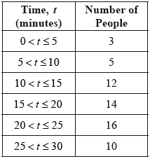
Write down the total number of people who were surveyed.[1]
Write down the mid-interval value for the \(10 < t \leqslant 15\) group.[1]
Find an estimate of the mean time people took to drink their coffee.[2]
The information above has been rewritten as a cumulative frequency table.
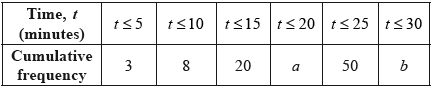
Write down the value of \(a\) and the value of \(b\).[2]
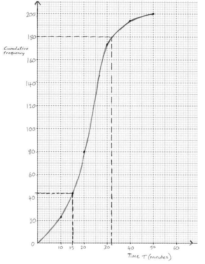
This information is shown in the following cumulative frequency graph.
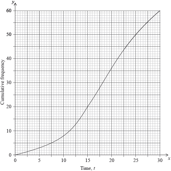
For the people who were surveyed, use the graph to estimate
(i) the time taken for the first \(40\) people to drink their coffee;
(ii) the number of people who take less than \(8\) minutes to drink their coffee;
(iii) the number of people who take more than \(23\) minutes to drink their coffee.[4]
Answer/Explanation
Markscheme
\(60\) (A1)[1 mark]
\(12.5\) (A1)[1 mark]
\(\frac{{3 \times 2.5 + 5 \times 7.5 + \ldots + 10 \times 27.5}}{{60}}\) (M1)
Note: Award (M1) for an attempt to substitute their mid-interval values (consistent with their answer to part (b)) into the formula for the mean.
Award (M1) where a table is constructed with their (consistent) mid-interval values listed along with the frequencies.
\( = \frac{{1075}}{{60}}{\text{ }}\left( {\frac{{215}}{{12}},{\text{ 17.9, 17.9166}} \ldots } \right)\) (A1)(ft)(G2)
Note: Follow through from their answer to part (b).[2 marks]
\(a = 34,{\text{ }}b = 60\) (A1)(A1)[2 marks]
(i) \( \leqslant {\text{21.25 minutes}}\) (A1)
Note: Accept \(21.25\).
Accept any answer between \(21\) and \(21.5\).
(Accept 21.5, but do not accept 21.)
(ii) \(5\) (A1)
Note: Accept \( < 6\). Do not accept \(6\).
Answer must be an integer.
(iii) \(60 – 45\) (M1)
\( = 15\) (A1)(G2)
Notes: Award (M1) for subtraction from \(60\). Accept \(15 \pm 1\).
Answer must be an integer.[4 marks]
Question
The cumulative frequency graph shows the speed, \(s\), in \({\text{km}}\,{{\text{h}}^{ – 1}}\), of \(120\) vehicles passing a hospital gate.
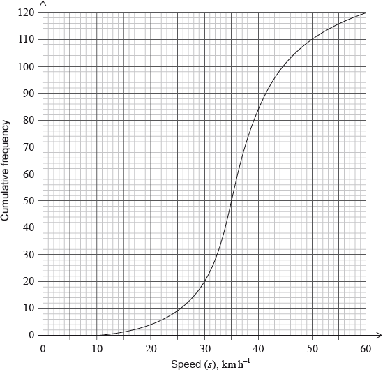
Estimate the minimum possible speed of one of these vehicles passing the hospital gate.[1]
Find the median speed of the vehicles.[2]
Write down the \({75^{{\text{th}}}}\) percentile.[1]
Calculate the interquartile range.[2]
The speed limit past the hospital gate is \(50{\text{ km}}\,{{\text{h}}^{ – 1}}\).
Find the number of these vehicles that exceed the speed limit.[2]
The table shows the speeds of these vehicles travelling past the hospital gate.
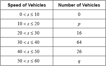
Find the value of \(p\) and of \(q\).[2]
The table shows the speeds of these vehicles travelling past the hospital gate.
(i) Write down the modal class.
(ii) Write down the mid-interval value for this class.[2]
The table shows the speeds of these vehicles travelling past the hospital gate.
Use your graphic display calculator to calculate an estimate of
(i) the mean speed of these vehicles;
(ii) the standard deviation.[3]
It is proposed that the speed limit past the hospital gate is reduced to \(40{\text{ km}}\,{{\text{h}}^{ – 1}}\) from the current \(50{\text{ km}}\,{{\text{h}}^{ – 1}}\).
Find the percentage of these vehicles passing the hospital gate that do not exceed the current speed limit but would exceed the new speed limit.[2]
Answer/Explanation
Markscheme
\(10{\text{ (km}}\,{{\text{h}}^{ – 1}})\) (A1)
\(36\) (G2)
\(41.5\) (G1)
\(41.5 – 32.5\) (M1)
\( = 9{\text{ (}} \pm {\text{1)}}\) (A1)(ft)(G2)
Notes: Award (M1) for quartiles seen. Follow through from part (c).
\(120 – 110\) (M1)
\( = 10\) (A1)(G2)
Note: Award (M1) for \(110\) seen.
\(p = 4\;\;\;q = 10\) (A1)(ft)(A1)(ft)
Note: Follow through from part (e).
(i) \(30 < s \leqslant 40\) (A1)
(ii) \(35\) (A1)(ft)
Note: Follow through from part (g)(i).
(i) \(36.8{\text{ (km}}\,{{\text{h}}^{ – 1}})\;\;\;(36.8333)\) (G2)(ft)
Notes: Follow through from part (f).
(ii) \(8.85\;\;\;(8.84904 \ldots )\) (G1)(ft)
Note: Follow through from part (f), irrespective of working seen.
\(\frac{{26}}{{120}} \times 100\) (M1)
Note: Award (M1) for \(\frac{{26}}{{120}} \times 100\) seen.
\( = 21.7{\text{ (}}\% )\;\;\;\left( {21.6666 \ldots ,{\text{ }}21\frac{2}{3},{\text{ }}\frac{{65}}{3}} \right)\) (A1)(G2)
Question
Daniel grows apples and chooses at random a sample of 100 apples from his harvest.
He measures the diameters of the apples to the nearest cm. The following table shows the distribution of the diameters.
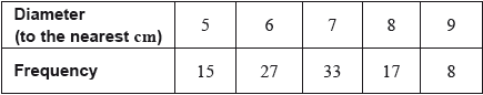
Using your graphic display calculator, write down the value of
(i) the mean of the diameters in this sample;
(ii) the standard deviation of the diameters in this sample.[3]
Daniel assumes that the diameters of all of the apples from his harvest are normally distributed with a mean of 7 cm and a standard deviation of 1.2 cm. He classifies the apples according to their diameters as shown in the following table.

Calculate the percentage of small apples in Daniel’s harvest.[3]
Daniel assumes that the diameters of all of the apples from his harvest are normally distributed with a mean of 7 cm and a standard deviation of 1.2 cm. He classifies the apples according to their diameters as shown in the following table.
Of the apples harvested, 5% are large apples.
Find the value of \(a\).[2]
Daniel assumes that the diameters of all of the apples from his harvest are normally distributed with a mean of 7 cm and a standard deviation of 1.2 cm. He classifies the apples according to their diameters as shown in the following table.
Find the percentage of medium apples.[2]
Daniel assumes that the diameters of all of the apples from his harvest are normally distributed with a mean of 7 cm and a standard deviation of 1.2 cm. He classifies the apples according to their diameters as shown in the following table.
This year, Daniel estimates that he will grow \({\text{100}}\,{\text{000}}\) apples.
Estimate the number of large apples that Daniel will grow this year.[2]
Answer/Explanation
Markscheme
(i) \(6.76{\text{ (cm)}}\) (G2)
Notes: Award (M1) for an attempt to use the formula for the mean with a least two rows from the table.
(ii) \(1.14{\text{ (cm)}}\;\;\;\left( {1.14122 \ldots {\text{ (cm)}}} \right)\) (G1)
\({\text{P}}({\text{diameter}} < 6.5) = 0.338\;\;\;(0.338461)\) (M1)(A1)
Notes: Award (M1) for attempting to use the normal distribution to find the probability or for correct region indicated on labelled diagram. Award (A1) for correct probability.
\(33.8(\% )\) (A1)(ft)(G3)
Notes: Award (A1)(ft) for converting their probability into a percentage.
\({\text{P}}({\text{diameter}} \geqslant a) = 0.05\) (M1)
Note: Award (M1) for attempting to use the normal distribution to find the probability or for correct region indicated on labelled diagram.
\(a = 8.97{\text{ (cm)}}\;\;\;(8.97382 \ldots )\) (A1)(G2)
\(100 – (5 + 33.8461 \ldots )\) (M1)
Note: Award (M1) for subtracting “\(5+\) their part (b)” from 100 or (M1) for attempting to use the normal distribution to find the probability \({\text{P}}\left( {6.5 \leqslant {\text{diameter}} < {\text{their part (c)}}} \right)\) or for correct region indicated on labelled diagram.
\( = 61.2(\% )\;\;\;\left( {61.1538 \ldots (\% )} \right)\) (A1)(ft)(G2)
Notes: Follow through from their answer to part (b). Percentage symbol is not required. Accept \(61.1(\%)\) (\(61.1209\ldots(\%)\)) if \(8.97\) used.
\(100\,000 \times 0.05\) (M1)
Note: Award (M1) for multiplying by \(0.05\) (or \(5\%\)).
\( = 5000\) (A1)(G2)
Question
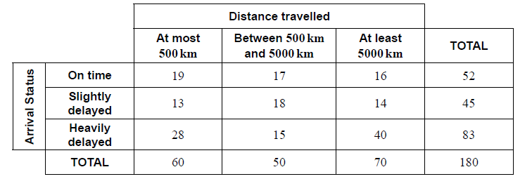
On one day 180 flights arrived at a particular airport. The distance travelled and the arrival status for each incoming flight was recorded. The flight was then classified as on time, slightly delayed, or heavily delayed.
The results are shown in the following table.
A χ2 test is carried out at the 10 % significance level to determine whether the arrival status of incoming flights is independent of the distance travelled.
The critical value for this test is 7.779.
A flight is chosen at random from the 180 recorded flights.
State the alternative hypothesis.[1]
Calculate the expected frequency of flights travelling at most 500 km and arriving slightly delayed.[2]
Write down the number of degrees of freedom.[1]
Write down the χ2 statistic.[2]
Write down the associated p-value.[1]
State, with a reason, whether you would reject the null hypothesis.[2]
Write down the probability that this flight arrived on time.[2]
Given that this flight was not heavily delayed, find the probability that it travelled between 500 km and 5000 km.[2]
Two flights are chosen at random from those which were slightly delayed.
Find the probability that each of these flights travelled at least 5000 km.[3]
Answer/Explanation
Markscheme
The arrival status is dependent on the distance travelled by the incoming flight (A1)
Note: Accept “associated” or “not independent”.[1 mark]
\(\frac{{60 \times 45}}{{180}}\) OR \(\frac{{60}}{{180}} \times \frac{{45}}{{180}} \times 180\) (M1)
Note: Award (M1) for correct substitution into expected value formula.
= 15 (A1) (G2)[2 marks]
4 (A1)
Note: Award (A0) if “2 + 2 = 4” is seen.[1 mark]
9.55 (9.54671…) (G2)
Note: Award (G1) for an answer of 9.54.[2 marks]
0.0488 (0.0487961…) (G1)[1 mark]
Reject the Null Hypothesis (A1)(ft)
Note: Follow through from their hypothesis in part (a).
9.55 (9.54671…) > 7.779 (R1)(ft)
OR
0.0488 (0.0487961…) < 0.1 (R1)(ft)
Note: Do not award (A1)(ft)(R0)(ft). Follow through from part (d). Award (R1)(ft) for a correct comparison, (A1)(ft) for a consistent conclusion with the answers to parts (a) and (d). Award (R1)(ft) for χ2calc > χ2crit , provided the calculated value is explicitly seen in part (d)(i).[2 marks]
\(\frac{{52}}{{180}}\,\,\left( {0.289,\,\,\frac{{13}}{{45}},\,\,28.9\,{\text{% }}} \right)\) (A1)(A1) (G2)
Note: Award (A1) for correct numerator, (A1) for correct denominator.[2 marks]
\(\frac{{35}}{{97}}\,\,\left( {0.361,\,\,36.1\,{\text{% }}} \right)\) (A1)(A1) (G2)
Note: Award (A1) for correct numerator, (A1) for correct denominator.[2 marks]
\(\frac{{14}}{{45}} \times \frac{{13}}{{44}}\) (A1)(M1)
Note: Award (A1) for two correct fractions and (M1) for multiplying their two fractions.
\( = \frac{{182}}{{1980}}\,\,\left( {0.0919,\,\,\frac{{91}}{{990}},\,0.091919 \ldots ,\,9.19\,{\text{% }}} \right)\) (A1) (G2)[3 marks]
Question
A transportation company owns 30 buses. The distance that each bus has travelled since being purchased by the company is recorded. The cumulative frequency curve for these data is shown.
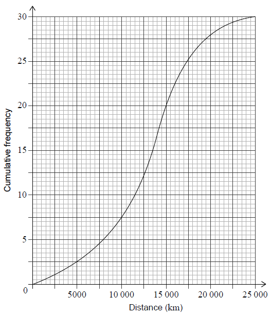
It is known that 8 buses travelled more than m kilometres.
Find the number of buses that travelled a distance between 15000 and 20000 kilometres.[2]
Use the cumulative frequency curve to find the median distance.[2]
Use the cumulative frequency curve to find the lower quartile.[1]
Use the cumulative frequency curve to find the upper quartile.[1]
Hence write down the interquartile range.[1]
Write down the percentage of buses that travelled a distance greater than the upper quartile.[1]
Find the number of buses that travelled a distance less than or equal to 12 000 km.[1]
Find the value of m.[2]
The smallest distance travelled by one of the buses was 2500 km.
The longest distance travelled by one of the buses was 23 000 km.
On graph paper, draw a box-and-whisker diagram for these data. Use a scale of 2 cm to represent 5000 km.[4]
Answer/Explanation
Markscheme
28 − 20 (A1)
Note: Award (A1) for 28 and 20 seen.
8 (A1)(G2)[2 marks]
13500 (G2)
Note: Accept an answer in the range 13500 to 13750.[2 marks]
10000 (G1)
Note: Accept an answer in the range 10000 to 10250.[1 mark]
16000 (G1)
Note: Accept an answer in the range 16000 to 16250.[1 mark]
6000 (A1)(ft)
Note: Follow through from their part (b)(ii) and (iii).[1 mark]
25% (A1)[1 mark]
11 (G1)[1 mark]
30 − 8 OR 22 (M1)
Note: Award (M1) for subtracting 30 − 8 or 22 seen.
15750 (A1)(G2)
Note: Accept 15750 ± 250.[2 marks]
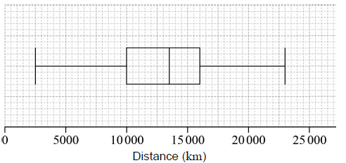 (A1)(A1)(A1)(A1)
Note: Award (A1) for correct label and scale; accept “distance” or “km” for label.
(A1)(ft) for correct median,
(A1)(ft) for correct quartiles and box,
(A1) for endpoints at 2500 and 23 000 joined to box by straight lines.
Accept ±250 for the median, quartiles and endpoints.
Follow through from their part (b).
The final (A1) is not awarded if the line goes through the box.[4 marks]