Question
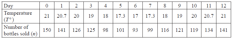
The number of bottles of water sold at a railway station on each day is given in the following table.
Write down
(i) the mean temperature;
(ii) the standard deviation of the temperatures.[2]
Write down the correlation coefficient, \(r\), for the variables \(n\) and \(T\).[1]
Comment on your value for \(r\).[2]
The equation of the line of regression for \(n\) on \(T\) is \(n = dT – 100\).
(i) Write down the value of \(d\).
(ii) Estimate how many bottles of water will be sold when the temperature is \({19.6^ \circ }\).[2]
On a day when the temperature was \({36^ \circ }\) Peter calculates that \(314\) bottles would be sold. Give one reason why his answer might be unreliable.[1]
Answer/Explanation
Markscheme
(i) 19.2 (G1)
(ii) 1.45 (G1)[2 marks]
\(r = 0.942\) (G1)[1 mark]
Strong, positive correlation. (A1)(ft)(A1)(ft)[2 marks]
(i) \(d = 11.5\) (G1)
(ii) \(n = 11.5 \times 19.6 – 100\)
\( = 125\) (accept \(126\)) (A1)(ft)
Note: Answer must be a whole number.[2 marks]
It is unreliable to extrapolate outside the values given (outlier). (R1)[1 mark]
Question
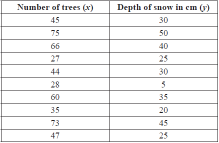
In a mountain region there appears to be a relationship between the number of trees growing in the region and the depth of snow in winter. A set of 10 areas was chosen, and in each area the number of trees was counted and the depth of snow measured. The results are given in the table below.
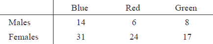
In a study on \(100\) students there seemed to be a difference between males and females in their choice of favourite car colour. The results are given in the table below. A \(\chi^2\) test was conducted.
Use your graphic display calculator to find the mean number of trees.[1]
Use your graphic display calculator to find the mean depth of snow.[1]
Use your graphic display calculator to find the standard deviation of the depth of snow.[1]
The covariance, Sxy = 188.5.
Write down the product-moment correlation coefficient, r.[2]
Write down the equation of the regression line of y on x.[2]
If the number of trees in an area is 55, estimate the depth of snow.[2]
Use the equation of the regression line to estimate the depth of snow in an area with 100 trees.[1]
Decide whether the answer in (e)(i) is a valid estimate of the depth of snow in the area. Give a reason for your answer.[2]
Write down the total number of male students.[1]
Show that the expected frequency for males, whose favourite car colour is blue, is 12.6.[2]
The calculated value of \({\chi ^2}\) is \(1.367\) and the critical value of \({\chi ^2}\) is \(5.99\) at the \(5\%\) significance level.
Write down the null hypothesis for this test.[1]
The calculated value of \({\chi ^2}\) is \(1.367\) and the critical value of \({\chi ^2}\) is \(5.99\) at the \(5\%\) significance level.
Write down the number of degrees of freedom.[1]
The calculated value of \({\chi ^2}\) is \(1.367\) and the critical value of \({\chi ^2}\) is \(5.99\) at the \(5\%\) significance level.
Determine whether the null hypothesis should be accepted at the \(5\%\) significance level. Give a reason for your answer.[2]
Answer/Explanation
Markscheme
50 (G1)[1 mark]
30.5 (G1)[1 mark]
12.3 (G1)
Note: Award (A1)(ft) for 13.0 in (iv) but only if 17.7 seen in (a)(ii).[1 mark]
\(r = \frac{{188.5}}{{(16.79 \times 12.33)}}\) (M1)
Note: Award (M1) for using their values in the correct formula.
= 0.911 (accept 0.912, 0.910) (A1)(ft)(G2)[2 marks]
y = 0.669x − 2.95 (G1)(G1)
Note: Award (G1) for 0.669x, (G1) for −2.95. If the answer is not in the form of an equation, award at most (G1)(G0).[2 marks]
Depth = 0.669 × 55 − 2.95 (M1)
= 33.8 (A1)(ft)(G2)(ft)
Note: Follow through from their (c) even if no working seen.[2 marks]
64.0 (accept 63.95, 63.9) (A1)(ft)(G1)(ft)
Note: Follow through from their (c) even if no working seen.[1 mark]
It is not valid. It lies too far outside the values that are given. Or equivalent. (A1)(R1)
Note: Do not award (A1)(R0).[2 marks]
28 (A1)[1 mark]
\(\frac{{28 \times 45}}{{100}}\left( {\frac{{28}}{{100}} \times \frac{{45}}{{100}} \times 100} \right)\) (M1)(A1)(ft)
Note: Award (M1) for correct formula, (A1) for correct substitution.
= 12.6 (AG)
Note: Do not award (A1) unless 12.6 seen.[2 marks]
the favourite car colour is independent of gender. (A1)
Note: Accept there is no association between gender and favourite car colour.
Do not accept ‘not related’ or ‘not correlated’.[1 mark]
\(2\) (A1)[1 marks]
Accept the null hypothesis since \(1.367 < 5.991\) (A1)(ft)(R1)
Note: Allow “Do not reject”. Follow through from their null hypothesis and their critical value.
Full credit for use of \(p\)-values from GDC [\(p = 0.505\)].
Do not award (A1)(R0). Award (R1) for valid comparison.[2 marks]
Question
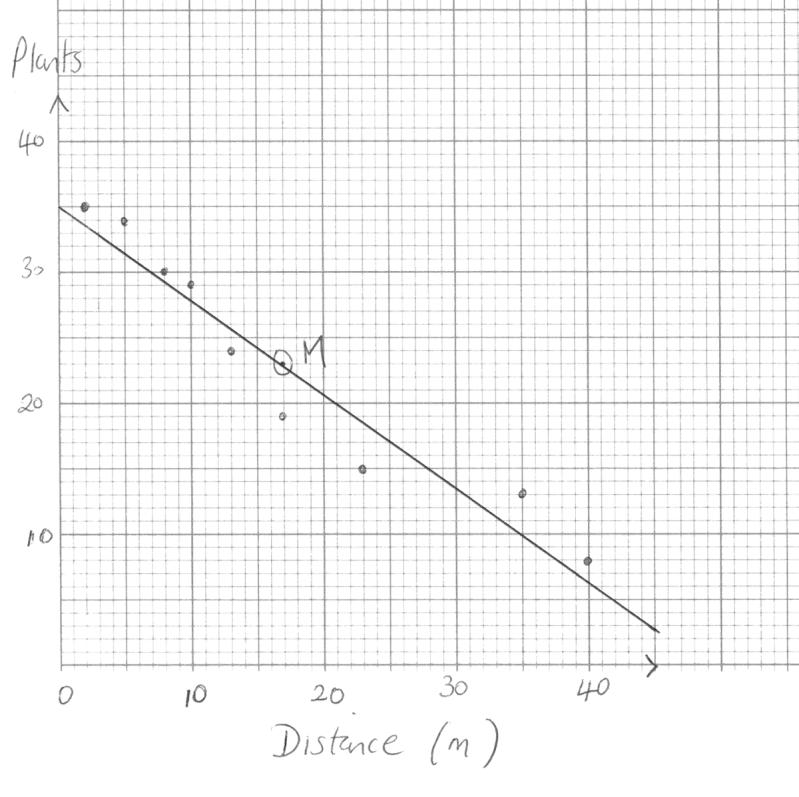
In an environmental study of plant diversity around a lake, a biologist collected data about the number of different plant species (y) that were growing at different distances (x) in metres from the lake shore.
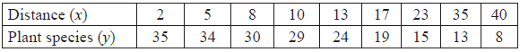
Draw a scatter diagram to show the data. Use a scale of 2 cm to represent 10 metres on the x-axis and 2 cm to represent 10 plant species on the y-axis.[4]
Using your scatter diagram, describe the correlation between the number of different plant species and the distance from the lake shore.[1]
Use your graphic display calculator to write down \(\bar x\), the mean of the distances from the lake shore.[1]
Use your graphic display calculator to write down \(\bar y\), the mean number of plant species.[1]
Plot the point (\(\bar x\), \(\bar y\)) on your scatter diagram. Label this point M.[2]
Write down the equation of the regression line y on x for the above data.[2]
Draw the regression line y on x on your scatter diagram.[2]
Estimate the number of plant species growing 30 metres from the lake shore.[2]
Answer/Explanation
Markscheme
 (A1)(A3)
Notes: Award (A1) for scales and labels (accept x/y).
Award (A3) for all points correct.
Award (A2) for 7 or 8 points correct.
Award (A1) for 5 or 6 points correct.
Award at most (A1)(A2) if points are joined up.
If axes are reversed award at most (A0)(A3)(ft).[4 marks]
Negative (A1)[1 mark]
17 (G1)[1 mark]
23 (G1)[1 mark]
Point correctly placed and labelled M (A1)(ft)(A1) Note: Accept an error of ±0.5.[2 marks]
y = –0.708x + 35.0 (G1)(G1)
Note: Award at most (G1)(G0) if y = not seen. Accept 35.[2 marks]
Regression line drawn that passes through M and (0, 35) (A1)(ft)(A1)(ft)
Note: Award (A1) for straight line that passes through M, (A1) for line (extrapolated if necessary) that passes through (0, 35) (accept error of ±1).
If ruler not used, award a maximum of (A1)(A0).[2 marks]
y = –0.708(30) + 35.0 (M1)
= 14 (Accept 13) (A1)(ft)(G2)
OR
Using graph: (M1) for some indication on graph of point, (A1)(ft) for answers. Final answer must be consistent with their graph. (M1)(A1)(ft)(G2)
Note: The final answer must be an integer.[2 marks]
Question
Alex and Kris are riding their bicycles together along a bicycle trail and note the following distance markers at the given times.
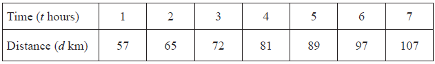
Draw a scatter diagram of the data. Use 1 cm to represent 1 hour and 1 cm to represent 10 km.[3]
Write down for this set of data the mean time, \(\bar t\).[1]
Write down for this set of data the mean distance, \(\bar d\).[1]
Mark and label the point \(M(\bar t,{\text{ }}\bar d)\) on your scatter diagram.[2]
Draw the line of best fit on your scatter diagram.[2]
Using your graph, estimate the time when Alex and Kris pass the 85 km distance marker. Give your answer correct to one decimal place.[2]
Write down the equation of the regression line for the data given.[2]
Using your equation calculate the distance marker passed by the cyclists at 10.3 hours.[2]
Is this estimate of the distance reliable? Give a reason for your answer.[2]
Answer/Explanation
Markscheme
 (A1)(A2)
Notes: Award (A1) for axes labelled with d and t and correct scale, (A2) for 6 or 7 points correctly plotted, (A1) for 4 or 5 points, (A0) for 3 or less points correctly plotted. Award at most (A1)(A1) if points are joined up. If axes are reversed award at most (A0)(A2)[3 marks]
\(\bar t = 4\) (G1)[1 mark]
\(\bar d = 81.1\left( {\frac{{568}}{7}} \right)\) (G1)
Note: If answers are the wrong way around award in (i) (G0) and in (ii) (G1)(ft).[1 mark]
Point marked and labelled with M or \(\bar t\), \(\bar d\) on their graph (A1)(ft)(A1)(ft)[2 marks]
Line of best fit drawn that passes through their M and (0, 48) (A1)(ft)(A1)(ft)
Notes: Award (A1)(ft) for straight line that passes through their M, (A1) for line (extrapolated if necessary) that passes through (0, 48).
Accept error of ±3. If ruler not used award a maximum of (A1)(ft)(A0).[2 marks]
4.5h (their answer ±0.2) (M1)(A1)(ft)(G2)
Note: Follow through from their graph. If method shown by some indication on graph of point but answer is incorrect, award (M1)(A0).[2 marks]
d = 8.25t + 48.1 (G1)(G1)
Notes: Award (G1) for 8.25, (G1) for 48.1.
Award at most (G1)(G0) if d = (or y =) is not seen.
Accept d – 81.1 = 8.25(t – 4) or equivalent.[2 marks]
d = 8.25 × 10.3 + 48.1 (M1)
d = 133 km (A1)(ft)(G2)[2 marks]
No (A1)
Outside the set of values of t or equivalent. (R1)
Note: Do not award (A1)(R0).[2 marks]
Question
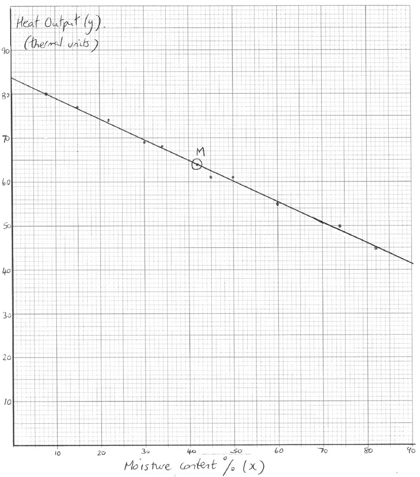
The heat output in thermal units from burning \(1{\text{ kg}}\) of wood changes according to the wood’s percentage moisture content. The moisture content and heat output of \(10\) blocks of the same type of wood each weighing \(1{\text{ kg}}\) were measured. These are shown in the table.
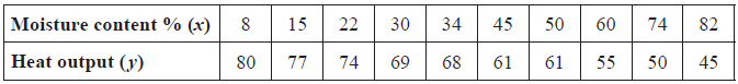
Draw a scatter diagram to show the above data. Use a scale of \(2{\text{ cm}}\) to represent \(10\% \) on the x-axis and a scale of \(2{\text{ cm}}\) to represent \(10\) thermal units on the y-axis.[4]
Write down
(i) the mean percentage moisture content, \(\bar x\) ;
(ii) the mean heat output, \(\bar y\) .[2]
Plot the point \((\bar x{\text{, }}\bar y)\) on your scatter diagram and label this point M .[2]
Write down the product-moment correlation coefficient, \(r\) .[2]
The equation of the regression line \(y\) on \(x\) is \(y = – 0.470x + 83.7\) . Draw the regression line \(y\) on \(x\) on your scatter diagram.[2]
The equation of the regression line \(y\) on \(x\) is \(y = – 0.470x + 83.7\) . Estimate the heat output in thermal units of a \(1{\text{ kg}}\) block of wood that has \(25\% \) moisture content.[2]
The equation of the regression line \(y\) on \(x\) is \(y = – 0.470x + 83.7\) . State, with a reason, whether it is appropriate to use the regression line \(y\) on \(x\) to estimate the heat output in part (f).[2]
Answer/Explanation
Markscheme
(A1) for correct scales and labels
(A3) for all ten points plotted correctly
(A2) for eight or nine points plotted correctly
(A1) for six or seven points plotted correctly (A4)
Note: Award at most (A0)(A3) if axes reversed.[4 marks]
(i) \(\bar x = 42\) (A1)
(ii) \(\bar y = 64\) (A1)[2 marks]
\((\bar x{\text{, }}\bar y)\) plotted on graph and labelled, M (A1)(ft)(A1)
Note: Award (A1)(ft) for position, (A1) for label.[2 marks]
\( – 0.998\) (G2)
Note: Award (G1) for correct sign, (G1) for correct absolute value.[1 mark]
line on graph (A1)(ft)(A1)
Notes: Award (A1)(ft) for line through their M, (A1) for approximately correct intercept (allow between \(83\) and \(85\)). It is not necessary that the line is seen to intersect the \(y\)-axis. The line must be straight for any mark to be awarded.[2 marks]
\(y = – 0.470(25) + 83.7\) (M1)
Note: Award (M1) for substitution into formula or some indication of method on their graph. \(y = – 0.470(0.25) + 83.7\) is incorrect.
\( = 72.0\) (accept \(71.95\) and \(72\)) (A1)(ft)(G2)
Note: Follow through from graph only if they show working on their graph. Accept \(72 \pm 0.5\) .[2 marks]
Yes since \(25\% \) lies within the data set and \(r\) is close to \( – 1\) (R1)(A1)
Note: Accept Yes, since \(r\) is close to \( – 1\)
Note: Do not award (R0)(A1).[2 marks]
Question
Part A
A university required all Science students to study one language for one year. A survey was carried out at the university amongst the 150 Science students. These students all studied one of either French, Spanish or Russian. The results of the survey are shown below.
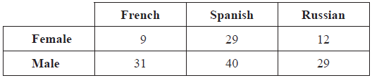
Ludmila decides to use the \({\chi ^2}\) test at the \(5\% \) level of significance to determine whether the choice of language is independent of gender.
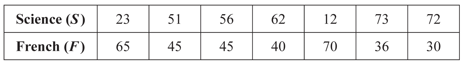
At the end of the year, only seven of the female Science students sat examinations in Science and French. The marks for these seven students are shown in the following table.
State Ludmila’s null hypothesis.[1]
Write down the number of degrees of freedom.[1]
Find the expected frequency for the females studying Spanish.[2]
Use your graphic display calculator to find the \({\chi ^2}\) test statistic for this data.[2]
State whether Ludmila accepts the null hypothesis. Give a reason for your answer.[2]
Draw a labelled scatter diagram for this data. Use a scale of \(2{\text{ cm}}\) to represent \(10{\text{ marks}}\) on the \(x\)-axis (\(S\)) and \(10{\text{ marks}}\) on the \(y\)-axis (\(F\)).[4]
Use your graphic calculator to find
(i) \({\bar S}\), the mean of \(S\) ;
(ii) \({\bar F}\), the mean of \(F\) .[2]
Plot the point \({\text{M}}(\bar S{\text{, }}\bar F)\) on your scatter diagram.[1]
Use your graphic display calculator to find the equation of the regression line of \(F\) on \(S\) .[2]
Draw the regression line on your scatter diagram.[2]
Carletta’s mark on the Science examination was \(44\). She did not sit the French examination.
Estimate Carletta’s mark for the French examination.[2]
Monique’s mark on the Science examination was 85. She did not sit the French examination. Her French teacher wants to use the regression line to estimate Monique’s mark.
State whether the mark obtained from the regression line for Monique’s French examination is reliable. Justify your answer.[2]
Answer/Explanation
Markscheme
\({{\text{H}}_0}:\) Choice of language is independent of gender. (A1)
Notes: Do not accept “not related” or “not correlated”.[1 mark]
\(2\) (A1)[1 mark]
\(\frac{{50 \times 69}}{{150}} = 23\) (M1)(A1)(G2)
Notes: Award (M1) for correct substituted formula, (A1) for \(23\).[2 marks]
\({\chi ^2} = 4.77\) (G2)
Notes: If answer is incorrect, award (M1) for correct substitution in the correct formula (all terms).[2 marks]
Accept \({{\text{H}}_0}\) since
\({\chi ^2}_{calc} < {\chi ^2}_{crit}(5.99)\) or \(p\)-value \((0.0923) > 0.05\) (R1)(A1)(ft)
Notes: Do not award (R0)(A1). Follow through from their (d) and (b).
Award (A1) for correct scale and labels.
Award (A3) for all seven points plotted correctly, (A2) for 5 or 6 points plotted correctly, (A1) for 3 or 4 points plotted correctly.
(A4)[4 marks]
(i) \({\bar S}= 49.9\), (G1)
(ii) \({\bar F} = 47.3\) (G1) [2 marks]
\({\text{M}}(49.9{\text{, }}47.3)\) plotted on scatter diagram (A1)(ft)
Notes: Follow through from (a) and (b).[1 mark]
\(F = – 0.619S + 78.2\) (G1)(G1)
Notes: Award (G1) for \( – 0.619S\), (G1) for \(78.2\). If the answer is not in the form of an equation, award (G1)(G0). Accept \(y = – 0.619x + 78.2\) .
OR
(F – 47.3 = – 0.619(S – 49.9)) (G1)(G1)
Note: Award (G1) for \( – 0.619\), (G1) for the coordinates of their midpoint used. Follow through from their values in (b).[2 marks]
line drawn on scatter diagram (A1)(ft)(A1)(ft)
Notes: The drawn line must be straight for any marks to be awarded. Award (A1)(ft) passing through their M plotted in (c). Award (A1)(ft) for correct \(y\)-intercept. Follow through from their \(y\)-intercept found in (d).[2 marks]
\(F = – 0.619 \times 44 + 78.2\) (M1)
\(= 51.0\) (allow \(51\) or \(50.9\)) (A1)(ft)(G2)(ft)
Note: Follow through from their equation.
OR
(M1) any indication of an acceptable graphical method. (M1)
(A1)(ft) from their regression line. (A1)(ft)(G2)(ft)[2 marks]
not reliable (A1)
Monique’s score in Science is outside the range of scores used to create the regression line. (R1)
Note: Do not award (A1)(R0).[2 marks]
Question
The table below shows the scores for 12 golfers for their first two rounds in a local golf tournament.
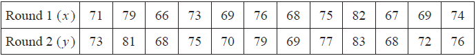
(i) Write down the mean score in Round 1.
(ii) Write down the standard deviation in Round 1.
(iii) Find the number of these golfers that had a score of more than one standard deviation above the mean in Round 1.[5]
Write down the correlation coefficient, r.[2]
Write down the equation of the regression line of y on x.[2]
Another golfer scored 70 in Round 1.
Calculate an estimate of his score in Round 2.[2]
Another golfer scored 89 in Round 1.
Determine whether you can use the equation of the regression line to estimate his score in Round 2. Give a reason for your answer.[2]
Answer/Explanation
Markscheme
(i) \(\frac{{71 + 79 + …}}{{12}}\) (M1)
\(72.4\left( {72.4166…,{\text{ }}\frac{{869}}{{12}}} \right)\) (A1)(G2)
Note: Award (M1) for correct substitution into the mean formula.
(ii) 4.77 (4.76896…) (G1)
(iii) 72.4 + 4.77 = 77.17 (M1)
Note: Award (M1) for adding their mean to their standard deviation.
Two golfers (A1)(ft)(G2)
Note: Follow through from their answers to parts (i) and (ii).[5 marks]
0.990 (0.99014…) (G2)[2 marks]
y = 1.01x + 0.816 (y = 1.01404…x + 0.81618…) (G1)(G1)
Notes: Award (G1) for 1.01x and (G1) for 0.816. If the answer is not an equation award a maximum of (G1)(G0).
OR
y − 74.25 = 1.01(x − 72.4)(y − 74.25 = 1.01404…(x − 72.4166…)) (A1)(A1)
Notes: Award (A1) for 1.01 correctly substituted in the equation, and (A1)(ft) for correct substitution of (72.4, 74.25) in the equation. Follow through from their part (a)(i). If the final answer is not an equation award a maximum of (A1)(A0).[2 marks]
y = 1.01404… × 70 + 0.81618… (M1)
Note: Award (M1) for substitution of 70 into their regression line equation from part (c).
y = 72 (71.7989…) (A1)(ft)(G2)
Note: Follow through from their part (c).[2 marks]
No, equation cannot be (reliably) used as 89 is outside the data range. (A1)(R1)
OR
Yes, but the result is not valid/not reliable as 89 is outside the data range/as we extrapolate (A1)(R1)
Note: Do not award (A1)(R0).[2 marks]
Question
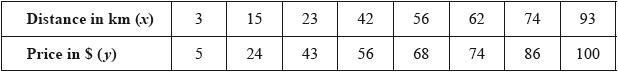
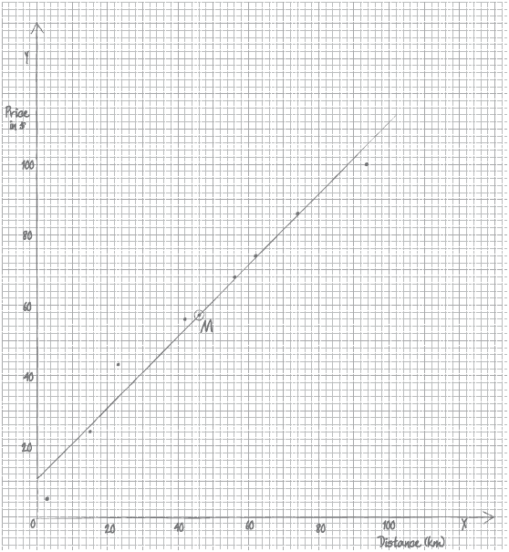
The table shows the distance, in km, of eight regional railway stations from a city centre terminus and the price, in \($\), of a return ticket from each regional station to the terminus.
Draw a scatter diagram for the above data. Use a scale of \(1\) cm to represent \(10\) km on the \(x\)-axis and \(1\) cm to represent \(\$10\) on the \(y\)-axis.[4]
Use your graphic display calculator to find
(i) \(\bar x\), the mean of the distances;
(ii) \(\bar y\), the mean of the prices.[2]
Plot and label the point \({\text{M }}(\bar x,{\text{ }}\bar y)\) on your scatter diagram.[1]
Use your graphic display calculator to find
(i) the product–moment correlation coefficient, \(r\,;\)
(ii) the equation of the regression line \(y\) on \(x\).[3]
Draw the regression line \(y\) on \(x\) on your scatter diagram.[2]
A ninth regional station is \(76\) km from the city centre terminus.
Use the equation of the regression line to estimate the price of a return ticket to the city centre terminus from this regional station. Give your answer correct to the nearest \({\mathbf{\$ }}\).[3]
Give a reason why it is valid to use your regression line to estimate the price of this return ticket.[1]
The actual price of the return ticket is \(\$80\).
Using your answer to part (f), calculate the percentage error in the estimated price of the ticket.[2]
Answer/Explanation
Markscheme
 (A4)
(A4)
Notes: Award (A1) for correct scale and labels (accept \(x\) and \(y\)).
Award (A3) for \(7\) or \(8\) points plotted correctly.
Award (A2) for \(5\) or \(6\) points plotted correctly.
Award (A1) for \(3\) or \(4\) points plotted correctly.
Award at most (A1)(A2) if points are joined up.
If axes are reversed, award at most (A0)(A3).
If graph paper is not used, award at most (A1)(A0).[4 marks]
(i) \((\bar x = ){\text{ 46}}\) (G1)
(ii) \((\bar y = ){\text{ 57}}\) (G1)[2 marks]
\({\text{M}} (46, 57)\) plotted and labelled on the scatter diagram (A1)(ft)
Notes: Follow through from their part (b).
Accept \((\bar x,{\text{ }}\bar y)\) as the label.[1 mark]
(i) \(0.986\) \((0.986322…)\) (G1)
(ii) \(y = 1.01x + 10.3\) \((y = 1.01431 \ldots x + 10.3412 \ldots )\) (G1)(G1)
Notes: Award (G1) for \(1.01x\), (G1) for \(10.3\).
Award (G1)(G0) if not written in the form of an equation.
OR
\((y – 57) = 1.01(x – 46)\) \(\left( {y – 57 = 1.01431…(x – 46)} \right)\) (G1)(G1)(ft)
Note: Award (G1) for \(1.01\), (G1) for their \(57\) and \(46\).[3 marks]
straight line drawn on the scatter diagram (A1)(ft)(A1)(ft)
Notes: The line must be straight for either of the two marks to be awarded.
Award (A1)(ft) passing through their \({\text{M}}\) plotted in (c).
Award (A1)(ft) for correct \(y\)-intercept (between \(9\) and \(12\)).
Follow through from their \(y\)-intercept found in part (d).
If part (d) is used, award (A1)(ft) for their intercept \(( \pm 1)\).[2 marks]
\(y = 1.01431… \times 76 + 10.3412…\) (M1)
Note: Award (M1) for substitution of \(76\) into their regression line.
\( = 87.4295…\) (A1)(ft)
Note: Follow through from part (d). If 3 sf values are used the value is \(87.06\).
\(\$87\) (A1)(ft)(G2)
Notes: The final (A1) is awarded for their answer given correct to the nearest dollar.
Method, followed by the answer of \(87\) earns (M1)(G2). It is not necessary to see the interim step.
Where the candidate uses their graph instead of the equation, and arrives at an answer other than \(87\), award, at most, (G1)(ft).
If the candidate uses their graph and arrives at the required answer of \(87\), award (G2)(ft).[3 marks]
\(76\) is within the range of distances given in the data OR the correlation coefficient is close to \(1\). (R1)
Notes: Award (R1) if either condition is given.
Sufficient to indicate that \(76\) is ‘within the data range’ and the correlation is ‘strong’.
Allow \({r^2}\) close to \(1\).
Do not accept “within the range of prices”.[1 mark]
\({\text{Percentage error}} = \frac{{87 – 80}}{{80}} \times 100\) (M1)
Note: Award (M1) for correct substitution into formula.
\(8.75\%\) (A1)(ft)(G2)
Notes: Follow through from their answer to part (f).
Accept either the rounded or unrounded answer to part (f).
If no integer value seen in part (f), follow through from their unrounded answer to part (f).
Answer must be positive.[2 marks]
Question
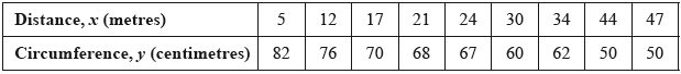
As part of his IB Biology field work, Barry was asked to measure the circumference of trees, in centimetres, that were growing at different distances, in metres, from a river bank. His results are summarized in the following table.
State whether distance from the river bank is a continuous or discrete variable.[1]
On graph paper, draw a scatter diagram to show Barry’s results. Use a scale of 1 cm to represent 5 m on the x-axis and 1 cm to represent 10 cm on the y-axis.[4]
Write down
(i) the mean distance, \(\bar x\), of the trees from the river bank;
(ii) the mean circumference, \(\bar y\), of the trees.[2]
Plot and label the point \({\text{M}}(\bar x,{\text{ }}\bar y)\) on your graph.[2]
Write down
(i) the Pearson’s product–moment correlation coefficient, \(r\), for Barry’s results;
(ii) the equation of the regression line \(y\) on \(x\), for Barry’s results.[4]
Draw the regression line \(y\) on \(x\) on your graph.[2]
Use the equation of the regression line \(y\) on \(x\) to estimate the circumference of a tree that is 40 m from the river bank.[2]
Answer/Explanation
Markscheme
continuous (A1)[1 mark]
 (A1)(A1)(A1)(A1)
Notes: Award (A1) for labelled axes and correct scales; if axes are reversed award (A0) and follow through for their points. Award (A1) for at least 3 correct points, (A2) for at least 6 correct points, (A3) for all 9 correct points. If scales are too small or graph paper has not been used, accuracy cannot be determined; award (A0). Do not penalize if extra points are seen.[4 marks]
(i) 26 (m) (A1)
(ii) 65 (cm) (A1)[2 marks]
point \({\text{M}}\) labelled, in correct position (A1)(A1)(ft)
Notes: Award (A1)(ft) for point plotted in correct position, (A1) for point labelled \({\text{M}}\) or \((\bar x,{\text{ }}\bar y)\). Follow through from their answers to part (c).[2 marks]
(i) \(-0.988\;{\text{ }}\left( {-0.988432 \ldots } \right)\) (G2)
Note: Award (G2) for \(-0.99\). Award (G1) for \(-0.990\).
Award (A1)(A0) if minus sign is omitted.
(ii) \(y = – 0.756x + 84.7\) \((y = – 0.756281 \ldots x + 84.6633 \ldots )\) (G2)
Notes: Award (A1) for \( – 0.756x\), (A1) for \(84.7\). If the answer is not given as an equation, award a maximum of (A1)(A0).[4 marks]
regression line through their \({\text{M}}\) (A1)((ft)
regression line through their \(\left( {0,85} \right)\) (accept \(85 \pm 1\)) (A1)(ft)
Notes: Follow through from part (d). Award a maximum of (A1)(A0) if the line is not straight. Do not penalize if either the line does not meet the y-axis or extends into quadrants other than the first.
If \({\text{M}}\) is not plotted or labelled, then follow through from part (c).
Follow through from their y-intercept in part (e)(ii).[2 marks]
\( – 0.756281(40) + 84.6633\) (M1)
\( = 54.4{\text{ (cm) }}(54.4120 \ldots )\) (A1)(ft)(G2)
Notes: Accept \(54.5\) (\(54.46\)) for use of 3 sf. Accept \(54.3\) from use of \(-0.76\) and \(84.7\).
Follow through from their equation in part (e)(ii) irrespective of working shown; the final answer seen must be consistent with that equation for the final (A1) to be awarded.
Do not accept answers taken from the graph.[2 marks]
Question
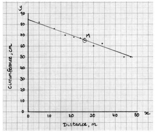
On one day 180 flights arrived at a particular airport. The distance travelled and the arrival status for each incoming flight was recorded. The flight was then classified as on time, slightly delayed, or heavily delayed.
The results are shown in the following table.
A χ2 test is carried out at the 10 % significance level to determine whether the arrival status of incoming flights is independent of the distance travelled.
The critical value for this test is 7.779.
A flight is chosen at random from the 180 recorded flights.
State the alternative hypothesis.[1]
Calculate the expected frequency of flights travelling at most 500 km and arriving slightly delayed.[2]
Write down the number of degrees of freedom.[1]
Write down the χ2 statistic.[2]
Write down the associated p-value.[1]
State, with a reason, whether you would reject the null hypothesis.[2]
Write down the probability that this flight arrived on time.[2]
Given that this flight was not heavily delayed, find the probability that it travelled between 500 km and 5000 km.[2]
Two flights are chosen at random from those which were slightly delayed.
Find the probability that each of these flights travelled at least 5000 km.[3]
Answer/Explanation
Markscheme
The arrival status is dependent on the distance travelled by the incoming flight (A1)
Note: Accept “associated” or “not independent”.[1 mark]
\(\frac{{60 \times 45}}{{180}}\) OR \(\frac{{60}}{{180}} \times \frac{{45}}{{180}} \times 180\) (M1)
Note: Award (M1) for correct substitution into expected value formula.
= 15 (A1) (G2)[2 marks]
4 (A1)
Note: Award (A0) if “2 + 2 = 4” is seen.[1 mark]
9.55 (9.54671…) (G2)
Note: Award (G1) for an answer of 9.54.[2 marks]
0.0488 (0.0487961…) (G1)[1 mark]
Reject the Null Hypothesis (A1)(ft)
Note: Follow through from their hypothesis in part (a).
9.55 (9.54671…) > 7.779 (R1)(ft)
OR
0.0488 (0.0487961…) < 0.1 (R1)(ft)
Note: Do not award (A1)(ft)(R0)(ft). Follow through from part (d). Award (R1)(ft) for a correct comparison, (A1)(ft) for a consistent conclusion with the answers to parts (a) and (d). Award (R1)(ft) for χ2calc > χ2crit , provided the calculated value is explicitly seen in part (d)(i).[2 marks]
\(\frac{{52}}{{180}}\,\,\left( {0.289,\,\,\frac{{13}}{{45}},\,\,28.9\,{\text{% }}} \right)\) (A1)(A1) (G2)
Note: Award (A1) for correct numerator, (A1) for correct denominator.[2 marks]
\(\frac{{35}}{{97}}\,\,\left( {0.361,\,\,36.1\,{\text{% }}} \right)\) (A1)(A1) (G2)
Note: Award (A1) for correct numerator, (A1) for correct denominator.[2 marks]
\(\frac{{14}}{{45}} \times \frac{{13}}{{44}}\) (A1)(M1)
Note: Award (A1) for two correct fractions and (M1) for multiplying their two fractions.
\( = \frac{{182}}{{1980}}\,\,\left( {0.0919,\,\,\frac{{91}}{{990}},\,0.091919 \ldots ,\,9.19\,{\text{% }}} \right)\) (A1) (G2)[3 marks]
Question
A transportation company owns 30 buses. The distance that each bus has travelled since being purchased by the company is recorded. The cumulative frequency curve for these data is shown.
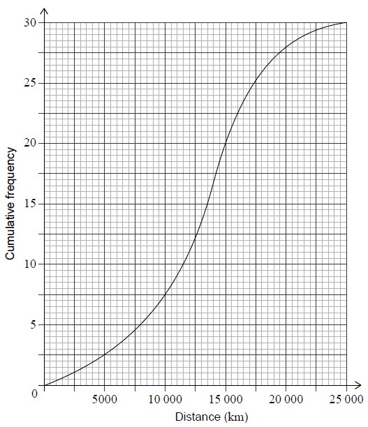
It is known that 8 buses travelled more than m kilometres.
Find the number of buses that travelled a distance between 15000 and 20000 kilometres.[2]
Use the cumulative frequency curve to find the median distance.[2]
Use the cumulative frequency curve to find the lower quartile.[1]
Use the cumulative frequency curve to find the upper quartile.[1]
Hence write down the interquartile range.[1]
Write down the percentage of buses that travelled a distance greater than the upper quartile.[1]
Find the number of buses that travelled a distance less than or equal to 12 000 km.[1]
Find the value of m.[2]
The smallest distance travelled by one of the buses was 2500 km.
The longest distance travelled by one of the buses was 23 000 km.
On graph paper, draw a box-and-whisker diagram for these data. Use a scale of 2 cm to represent 5000 km.[4]
Answer/Explanation
Markscheme
28 − 20 (A1)
Note: Award (A1) for 28 and 20 seen.
8 (A1)(G2)[2 marks]
13500 (G2)
Note: Accept an answer in the range 13500 to 13750.[2 marks]
10000 (G1)
Note: Accept an answer in the range 10000 to 10250.[1 mark]
16000 (G1)
Note: Accept an answer in the range 16000 to 16250.[1 mark]
6000 (A1)(ft)
Note: Follow through from their part (b)(ii) and (iii).[1 mark]
25% (A1)[1 mark]
11 (G1)[1 mark]
30 − 8 OR 22 (M1)
Note: Award (M1) for subtracting 30 − 8 or 22 seen.
15750 (A1)(G2)
Note: Accept 15750 ± 250.[2 marks]
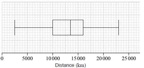 (A1)(A1)(A1)(A1)
Note: Award (A1) for correct label and scale; accept “distance” or “km” for label.
(A1)(ft) for correct median,
(A1)(ft) for correct quartiles and box,
(A1) for endpoints at 2500 and 23 000 joined to box by straight lines.
Accept ±250 for the median, quartiles and endpoints.
Follow through from their part (b).
The final (A1) is not awarded if the line goes through the box.[4 marks]