Question
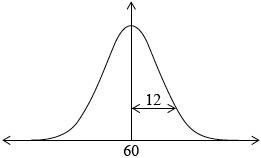
A group of candidates sat a Chemistry examination and a Physics examination. The candidates’ marks in the Chemistry examination are normally distributed with a mean of \(60\) and a standard deviation of \(12\).
Draw a diagram that shows this information.[2]
Write down the probability that a randomly chosen candidate who sat the Chemistry examination scored at most 60 marks.[1]
Hee Jin scored 80 marks in the Chemistry examination.
Find the probability that a randomly chosen candidate who sat the Chemistry examination scored more than Hee Jin.[2]
The candidates’ marks in the Physics examination are normally distributed with a mean of \(63\) and a standard deviation of \(10\). Hee Jin also scored \(80\) marks in the Physics examination.
Find the probability that a randomly chosen candidate who sat the Physics examination scored less than Hee Jin.[2]
The candidates’ marks in the Physics examination are normally distributed with a mean of \(63\) and a standard deviation of \(10\). Hee Jin also scored \(80\) marks in the Physics examination.
Determine whether Hee Jin’s Physics mark, compared to the other candidates, is better than her mark in Chemistry. Give a reason for your answer.[2]
To obtain a “grade A” a candidate must be in the top \(10\% \) of the candidates who sat the Physics examination.
Find the minimum possible mark to obtain a “grade A”. Give your answer correct to the nearest integer.[3]
Answer/Explanation
Markscheme
 (A1)(A1)
Notes: Award (A1) for rough sketch of normal curve centred at \(60\), (A1) for some indication of \(12\) as the standard deviation eg, as diagram, or with \(72\) and \(48\) shown on the horizontal axis in appropriate places, or for \(96\) and \(24\) shown on the horizontal axis in appropriate places.[2 marks]
\(0.5 \left( {\frac{1}{2},{\text{ 50% }}} \right)\) (A1)
Note: Accept only the exact answer.[1 mark]
\(0.0478{\text{ }} (0.0477903…)\) (G2)
Note: Award (G1) for \(0.952209…\), award (M1)(G0) for diagram with correct area shown but incorrect answer.[2 marks]
\(0.955 {\text{ }} (0.955434…)\) (G2)
Note: Award (G1) for \(0.044565…\), award (M1)(G0) for diagram with correct area shown but incorrect answer.[2 marks]
\(0.0446 < 0.0478\) (R1)
Notes: Award (R1) for correct comparison seen. Accept alternative methods, for example, \(1–\) (their answer to part (c)) used in comparison or a comparison based on \(z\) scores.
the Physics result is better (A1)(ft)
Notes: Do not award (R0)(A1). Follow through from their answers to part (c) and part (d).[2 marks]
\(76\) (G3)
Notes: Award (G1) for \(75.8155…\), award (G2) for \(75\).
Award (M1)(G0) for diagram with correct area shown but incorrect answer.[3 marks]
Question
Daniel grows apples and chooses at random a sample of 100 apples from his harvest.
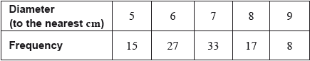
He measures the diameters of the apples to the nearest cm. The following table shows the distribution of the diameters.
Using your graphic display calculator, write down the value of
(i) the mean of the diameters in this sample;
(ii) the standard deviation of the diameters in this sample.[3]
Daniel assumes that the diameters of all of the apples from his harvest are normally distributed with a mean of 7 cm and a standard deviation of 1.2 cm. He classifies the apples according to their diameters as shown in the following table.

Calculate the percentage of small apples in Daniel’s harvest.[3]
Daniel assumes that the diameters of all of the apples from his harvest are normally distributed with a mean of 7 cm and a standard deviation of 1.2 cm. He classifies the apples according to their diameters as shown in the following table.
Of the apples harvested, 5% are large apples.
Find the value of \(a\).[2]
Daniel assumes that the diameters of all of the apples from his harvest are normally distributed with a mean of 7 cm and a standard deviation of 1.2 cm. He classifies the apples according to their diameters as shown in the following table.
Find the percentage of medium apples.[2]
Daniel assumes that the diameters of all of the apples from his harvest are normally distributed with a mean of 7 cm and a standard deviation of 1.2 cm. He classifies the apples according to their diameters as shown in the following table.
This year, Daniel estimates that he will grow \({\text{100}}\,{\text{000}}\) apples.
Estimate the number of large apples that Daniel will grow this year.[2]
Answer/Explanation
Markscheme
(i) \(6.76{\text{ (cm)}}\) (G2)
Notes: Award (M1) for an attempt to use the formula for the mean with a least two rows from the table.
(ii) \(1.14{\text{ (cm)}}\;\;\;\left( {1.14122 \ldots {\text{ (cm)}}} \right)\) (G1)
\({\text{P}}({\text{diameter}} < 6.5) = 0.338\;\;\;(0.338461)\) (M1)(A1)
Notes: Award (M1) for attempting to use the normal distribution to find the probability or for correct region indicated on labelled diagram. Award (A1) for correct probability.
\(33.8(\% )\) (A1)(ft)(G3)
Notes: Award (A1)(ft) for converting their probability into a percentage.
\({\text{P}}({\text{diameter}} \geqslant a) = 0.05\) (M1)
Note: Award (M1) for attempting to use the normal distribution to find the probability or for correct region indicated on labelled diagram.
\(a = 8.97{\text{ (cm)}}\;\;\;(8.97382 \ldots )\) (A1)(G2)
\(100 – (5 + 33.8461 \ldots )\) (M1)
Note: Award (M1) for subtracting “\(5+\) their part (b)” from 100 or (M1) for attempting to use the normal distribution to find the probability \({\text{P}}\left( {6.5 \leqslant {\text{diameter}} < {\text{their part (c)}}} \right)\) or for correct region indicated on labelled diagram.
\( = 61.2(\% )\;\;\;\left( {61.1538 \ldots (\% )} \right)\) (A1)(ft)(G2)
Notes: Follow through from their answer to part (b). Percentage symbol is not required. Accept \(61.1(\%)\) (\(61.1209\ldots(\%)\)) if \(8.97\) used.
\(100\,000 \times 0.05\) (M1)
Note: Award (M1) for multiplying by \(0.05\) (or \(5\%\)).
\( = 5000\) (A1)(G2)
Question
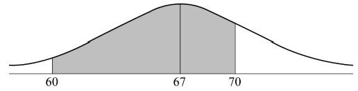
A speed camera on Peterson Road records the speed of each passing vehicle. The speeds are found to be normally distributed with a mean of \(67\,{\text{km}}\,{{\text{h}}^{ – 1}}\) and a standard deviation of \(3.4\,{\text{km}}\,{{\text{h}}^{ – 1}}\).
Sketch a diagram of this normal distribution and shade the region representing the probability that the speed of a vehicle is between \(60\) and \(70\,{\text{km}}\,{{\text{h}}^{ – 1}}\).[2]
A vehicle on Peterson Road is chosen at random.
Find the probability that the speed of this vehicle is
(i) more than \(60\,{\text{km}}\,{{\text{h}}^{ – 1}}\);
(ii) less than \(70\,{\text{km}}\,{{\text{h}}^{ – 1}}\);
(iii) between \(60\) and \(70\,{\text{km}}\,{{\text{h}}^{ – 1}}\).[3]
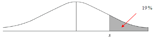
It is found that \(19\,\% \) of the vehicles are exceeding the speed limit of \(s\,{\text{km}}\,{{\text{h}}^{ – 1}}\).
Find the value of \(s\) , correct to the nearest integer.[2]
There is a fine of \({\text{US}}\$ 65\) for exceeding the speed limit on Peterson Road. On a particular day the total value of fines issued was \({\text{US}}\$ 14\,820\).
(i) Calculate the number of fines that were issued on this day.
(ii) Estimate the total number of vehicles that passed the speed camera on Peterson Road on this day.[4]
Answer/Explanation
Markscheme
(A1)(A1)
Note: Award (A1) for normal curve with mean of \(67\) indicated or two vertical lines drawn approximately in correct place. Award (A1) for correct shaded region (between the vertical lines.).
(i) \(0.980\,\,\,(0.980244…,\,\,98.0\,\% )\) (G1)
(ii) \(0.811\,\,\,(0.811207…,\,\,81.1\,\% )\) (G1)
(iii) \(0.791\,\,\,(0.791451…,\,\,79.1\,\% )\) (G1)
\({\text{P}}\,\left( {S > s} \right) = 19\,\% \,\,(0.19)\) OR \({\text{P}}\,\left( {S > s} \right) = 81\,\% \,\,(0.81)\) (M1)
OR
(M1)
Note: Award (M1) for the correct probability equation OR for a correct region indicated on labelled diagram.
\((s = )\,\,70.0\,\,\,(69.9848…)\) (A1)(G2)
Note: Award (M1) for any correct method.
(i) \(\frac{{14\,820}}{{65}}\) (M1)
Note: Award (M1) for dividing \(14\,820\) by \(65\).
\( = 228\) (A1)(G2)
(ii) \(\frac{{{\text{their 228}}}}{{0.19}}\) (or equivalent) (M1)
\( = 1200\) (vehicles) (A1)(ft)(G2)
Note: Award (M1) for correct method. Follow through from their part (d)(i).
Question
A manufacturer produces 1500 boxes of breakfast cereal every day.
The weights of these boxes are normally distributed with a mean of 502 grams and a standard deviation of 2 grams.
All boxes of cereal with a weight between 497.5 grams and 505 grams are sold. The manufacturer’s income from the sale of each box of cereal is $2.00.
The manufacturer recycles any box of cereal with a weight not between 497.5 grams and 505 grams. The manufacturer’s recycling cost is $0.16 per box.
A different manufacturer produces boxes of cereal with weights that are normally distributed with a mean of 350 grams and a standard deviation of 1.8 grams.
This manufacturer sells all boxes of cereal that are above a minimum weight, \(w\).
They sell 97% of the cereal boxes produced.
Draw a diagram that shows this information.[2]
(i) Find the probability that a box of cereal, chosen at random, is sold.
(ii) Calculate the manufacturer’s expected daily income from these sales.[4]
Calculate the manufacturer’s expected daily recycling cost.[2]
Calculate the value of \(w\).[3]
Answer/Explanation
Markscheme
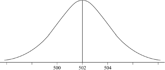
(A1)(A1)
Notes: Award (A1) for bell shape with mean of 502.
Award (A1) for an indication of standard deviation eg 500 and 504.[2 marks]
(i) \(0.921{\text{ }}(0.920968 \ldots ,{\text{ }}92.0968 \ldots \% )\) (G2)
Note: Award (M1) for a diagram showing the correct shaded region.
(ii) \(1500 \times 2 \times 0.920968 \ldots \) (M1)
\( = {\text{ }}(\$ ){\text{ }}2760{\text{ }}(2762.90 \ldots )\) (A1)(ft)(G2)
Note: Follow through from their answer to part (b)(i).[4 marks]
\(1500 \times 0.16 \times 0.079031 \ldots \) (M1)
Notes: Award (A1) for \(1500 \times 0.16 \times {\text{ their }}(1 – 0.920968 \ldots )\).
OR
\((1500 – 1381.45) \times 0.16\) (M1)
Notes: Award (M1) for \((1500 – {\text{their }}1381.45) \times 0.16\).
\( = (\$ )19.0{\text{ (}}18.9676 \ldots )\) (A1)(ft)(G2)[2 marks]
\(347{\text{ }}({\text{grams}}){\text{ }}(346.614 \ldots )\) (G3)
Notes: Award (G2) for an answer that rounds to 346.
Award (G1) for \(353.385 \ldots \) seen without working (for finding the top 3%).[3 marks]
Question
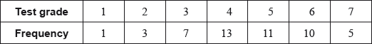
The table below shows the distribution of test grades for 50 IB students at Greendale School.
A student is chosen at random from these 50 students.
A second student is chosen at random from these 50 students.
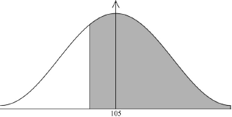
The number of minutes that the 50 students spent preparing for the test was normally distributed with a mean of 105 minutes and a standard deviation of 20 minutes.
Calculate the mean test grade of the students;[2]
Calculate the standard deviation.[1]
Find the median test grade of the students.[1]
Find the interquartile range.[2]
Find the probability that this student scored a grade 5 or higher.[2]
Given that the first student chosen at random scored a grade 5 or higher, find the probability that both students scored a grade 6.[3]
Calculate the probability that a student chosen at random spent at least 90 minutes preparing for the test.[2]
Calculate the expected number of students that spent at least 90 minutes preparing for the test.[2]
Answer/Explanation
Markscheme
\(\frac{{1(1) + 3(2) + 7(3) + 13(4) + 11(5) + 10(6) + 5(7)}}{{50}} = \frac{{230}}{{50}}\) (M1)
Note: Award (M1) for correct substitution into mean formula.
\( = 4.6\) (A1) (G2)[2 marks]
\(1.46{\text{ }}(1.45602 \ldots )\) (G1)[1 mark]
5 (A1)[1 mark]
\(6 – 4\) (M1)
Note: Award (M1) for 6 and 4 seen.
\( = 2\) (A1) (G2)[2 marks]
\(\frac{{11 + 10 + 5}}{{50}}\) (M1)
Note: Award (M1) for \(11 + 10 + 5\) seen.
\( = \frac{{26}}{{50}}{\text{ }}\left( {\frac{{13}}{{25}},{\text{ }}0.52,{\text{ }}52\% } \right)\) (A1) (G2)[2 marks]
\(\frac{{10}}{{{\text{their }}26}} \times \frac{9}{{49}}\) (M1)(M1)
Note: Award (M1) for \(\frac{{10}}{{{\text{their }}26}}\) seen, (M1) for multiplying their first probability by \(\frac{9}{{49}}\).
OR
\(\frac{{\frac{{10}}{{50}} \times \frac{9}{{49}}}}{{\frac{{26}}{{50}}}}\)
Note: Award (M1) for \({\frac{{10}}{{50}} \times \frac{9}{{49}}}\) seen, (M1) for dividing their first probability by \(\frac{{{\text{their }}26}}{{50}}\).
\( = \frac{{45}}{{637}}{\text{ (}}0.0706,{\text{ }}0.0706436 \ldots ,{\text{ }}7.06436 \ldots \% )\) (A1)(ft) (G3)
Note: Follow through from part (d).[3 marks]
\({\text{P}}(X \geqslant 90)\) (M1)
OR
 (M1)
(M1)
Note: Award (M1) for a diagram showing the correct shaded region \(( > 0.5)\).
\(0.773{\text{ }}(0.773372 \ldots ){\text{ }}0.773{\text{ }}(0.773372 \ldots ,{\text{ }}77.3372 \ldots \% )\) (A1) (G2)[2 marks]
\(0.773372 \ldots \times 50\) (M1)
\( = 38.7{\text{ }}(38.6686 \ldots )\) (A1)(ft) (G2)
Note: Follow through from part (f)(i).[2 marks]
Question
The weight, W, of basketball players in a tournament is found to be normally distributed with a mean of 65 kg and a standard deviation of 5 kg.
The probability that a basketball player has a weight that is within 1.5 standard deviations of the mean is q.
A basketball coach observed 60 of her players to determine whether their performance and their weight were independent of each other. Her observations were recorded as shown in the table.
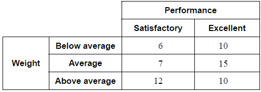
She decided to conduct a χ 2 test for independence at the 5% significance level.
Find the probability that a basketball player has a weight that is less than 61 kg.[2]
In a training session there are 40 basketball players.
Find the expected number of players with a weight less than 61 kg in this training session.[2]
Sketch a normal curve to represent this probability.[2]
Find the value of q.[1]
Given that P(W > k) = 0.225 , find the value of k.[2]
For this test state the null hypothesis.[1]
For this test find the p-value.[2]
State a conclusion for this test. Justify your answer.[2]
Answer/Explanation
Markscheme
P(W < 61) (M1)
Note: Award (M1) for correct probability statement.
OR
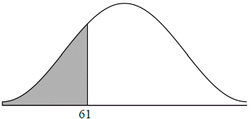 (M1)
(M1)
Note: Award (M1) for correct region labelled and shaded on diagram.
= 0.212 (0.21185…, 21.2%) (A1)(G2)[2 marks]
40 × 0.21185… (M1)
Note: Award (M1) for product of 40 and their 0.212.
= 8.47 (8.47421…) (A1)(ft)(G2)
Note: Follow through from their part (a)(i) provided their answer to part (a)(i) is less than 1.[2 marks]
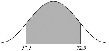 (A1)(M1)
Note: Award (A1) for two correctly labelled vertical lines in approximately correct positions. The values 57.5 and 72.5, or μ − 1.5σ and μ + 1.5σ are acceptable labels. Award (M1) for correctly shaded region marked by their two vertical lines.[2 marks]
0.866 (0.86638…, 86.6%) (A1)(ft)
Note: Follow through from their part (b)(i) shaded region if their values are clear.[1 mark]
P(W < k) = 0.775 (M1)
OR
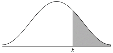 (M1)
(M1)
Note: Award (A1) for correct region labelled and shaded on diagram.
(k =) 68.8 (68.7770…) (A1)(G2)[2 marks]
(H0🙂 performance (of players) and (their) weight are independent. (A1)
Note: Accept “there is no association between performance (of players) and (their) weight”. Do not accept “not related” or “not correlated” or “not influenced”.[1 mark]
0.287 (0.287436…) (G2)[2 marks]
accept/ do not reject null hypothesis/H0 (A1)(ft)
OR
performance (of players) and (their) weight are independent. (A1)(ft)
0.287 > 0.05 (R1)(ft)
Note: Accept p-value>significance level provided their p-value is seen in b(ii). Accept 28.7% > 5%. Do not award (A1)(R0). Follow through from part (d).[2 marks]
Question
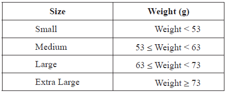
The Brahma chicken produces eggs with weights in grams that are normally distributed about a mean of \(55{\text{ g}}\) with a standard deviation of \(7{\text{ g}}\). The eggs are classified as small, medium, large or extra large according to their weight, as shown in the table below.
Sketch a diagram of the distribution of the weight of Brahma chicken eggs. On your diagram, show clearly the boundaries for the classification of the eggs.[3]
An egg is chosen at random. Find the probability that the egg is
(i) medium;
(ii) extra large.[4]
There is a probability of \(0.3\) that a randomly chosen egg weighs more than \(w\) grams.
Find \(w\) .[2]
The probability that a Brahma chicken produces a large size egg is \(0.121\). Frank’s Brahma chickens produce \(2000\) eggs each month.
Calculate an estimate of the number of large size eggs produced by Frank’s chickens each month.[2]
The selling price, in US dollars (USD), of each size is shown in the table below.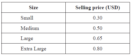
The probability that a Brahma chicken produces a small size egg is \(0.388\).
Estimate the monthly income, in USD, earned by selling the \(2000\) eggs. Give your answer correct to two decimal places.[3]
Answer/Explanation
Markscheme
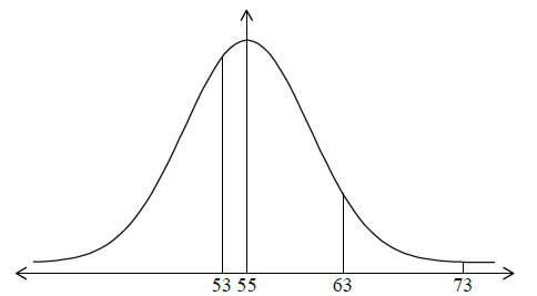
(A1) for normal curve with mean of \(55\) indicated
(A1) for three lines in approximately the correct position
(A1) for labels on the three lines (A1)(A1)(A1)
(i) \({\text{P}}(53 \leqslant {\text{Weight}} < 63) = 0.486\) (\(0.485902 \ldots \)) (M1)(A1)(G2)
Note: Award (M1) for correct region indicated on labelled diagram.
(ii) \({\text{P}}({\text{Weight}} > 73) = 0.00506\) (\(0.00506402\)) (M1)(A1)(G2)
Note: Award (M1) for correct region indicated on labelled diagram.
\({\text{P}}({\text{Weight}} > w) = 0.3\) (M1)
\(w = 58.7\) (\(58.6708 \ldots \)) (A1)(G2)
Note: Award (M1) for correct region indicated on labelled diagram.
Expected number of large size eggs
\( = 2000(0.121)\) (M1)
\( = 242\) (A1)(G2)
Expected income
\( = 2000 \times 0.30 \times 0.388 + 2000 \times 0.50 \times 0.486 + 2000 \times 0.65 \times 0.121 + 2000 \times 0.80 \times 0.00506\) (M1)(M1)
Note: Award (M1) for their correct products, (M1) for addition of 4 terms.
\( = 884.20{\text{ USD}}\) (A1)(ft)(G3)
Note: Follow through from part (b).