IB Mathematics SL 4.4 Linear correlation of bivariate data AI HL Paper 2- Exam Style Questions- New Syllabus

a
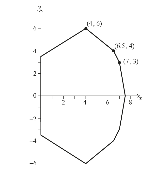
The cross-section follows a straight line from (0, 3.5) to (4, 6).
Slope \( m = \frac{6 – 3.5}{4 – 0} = \frac{2.5}{4} = 0.625 = \frac{5}{8} \).
Using point (0, 3.5): \( y – 3.5 = \frac{5}{8}×(x – 0) \), so \( y = \frac{5}{8}×x + 3.5 \).
Alternatively, using \( \frac{7}{2} = 3.5 \), the equation is \( y = \frac{5}{8}×x + \frac{7}{2} \).
Explanation:
Use the point-slope form with the given points to derive the linear equation.
Result:
\( y = \frac{5}{8}×x + \frac{7}{2} \) (or \( y = 0.625×x + 3.5 \))

b
b.(i) For least squares regression \( y = a×x^2 + b×x + c \) with points (4, 6), (6.5, 4), (7, 3), (7.5, 0), solve the normal equations.
Summing \( x \), \( x^2 \), \( x^3 \), \( x^4 \), and \( y \) over the points, approximate coefficients are \( a ≈ -0.97463 \), \( b ≈ 9.55919 \), \( c ≈ -16.6569 \), rounded to \( y = -0.975×x^2 + 9.5×x – 16.7 \).
b.(ii) Gradient \( \frac{dy}{dx} = -1.95×x + 9.5 \). At \( x = 4 \): \( -1.95 × 4 + 9.5 = -7.8 + 9.5 = 1.7 \), which is positive.
Since the curve should decrease from (4, 6) to (6.5, 4), a positive gradient suggests a poor fit at the junction.
Explanation:
Use least squares to fit the quadratic and calculate the gradient to assess model fit.
Result:
b.(i) \( y = -0.975×x^2 + 9.5×x – 16.7 \)
b.(ii) The gradient is positive at \( x = 4 \) (1.7), indicating a poor fit as the curve should decrease.

c
For a quadratic \( y = a×x^2 + b×x + c \) with maximum at (4, 6), the vertex \( x = -\frac{b}{2×a} = 4 \), so \( -b = 8×a \), \( b = -8×a \).
At vertex, \( y = 6 \), so \( 16×a – 32×a + c = 6 \), \( -16×a + c = 6 \).
Passes through (7.5, 0): \( 56.25×a – 60×a + c = 0 \), \( -3.75×a + c = 0 \).
Solve: \( c = 3.75×a \), substitute into \( -16×a + 3.75×a = 6 \), \( -12.25×a = 6 \), \( a = -\frac{6}{12.25} = -\frac{24}{49} \).
Then \( c = 3.75 × -\frac{24}{49} = -\frac{90}{49} \), \( b = -8 × -\frac{24}{49} = \frac{192}{49} \).
Thus, \( y = -\frac{24}{49}×x^2 + \frac{192}{49}×x – \frac{90}{49} \), or approximately \( y = -0.490×x^2 + 3.92×x – 1.84 \).
Explanation:
Derive the quadratic using vertex form and the given point, solving the system of equations step-by-step.
Result:
\( y = -\frac{24}{49}×x^2 + \frac{192}{49}×x – \frac{90}{49} \) (or \( y = -0.490×x^2 + 3.92×x – 1.84 \))

d
d.(i) Volume of revolution about x-axis uses \( V = \pi \int_a^b y^2 dx \).
For \( x \in [0, 4] \), \( y = \frac{5}{8}×x + \frac{7}{2} \); for \( x \in [4, 7.5] \), \( y = -\frac{24}{49}×(x – 4)^2 + 6 \).
Thus, \( V = \pi \int_0^4 \left(\frac{5}{8}×x + \frac{7}{2}\right)^2 dx + \pi \int_4^{7.5} \left(-\frac{24}{49}×(x – 4)^2 + 6\right)^2 dx \).
d.(ii) To estimate the volume, we use the disk method:
First integral (\( x \in [0, 4] \)):
Expand \( \left(\frac{5}{8}×x + \frac{7}{2}\right)^2 = \frac{25}{64}×x^2 + \frac{35}{8}×x + \frac{49}{4} \).
So \( \int_0^4 \left(\frac{25}{64}×x^2 + \frac{35}{8}×x + \frac{49}{4}\right) dx = \left[\frac{25}{64} × \frac{x^3}{3} + \frac{35}{8} × \frac{x^2}{2} + \frac{49}{4}×x\right]_0^4 \).
Evaluate at \( x = 4 \): \( \frac{25}{64} × \frac{64}{3} + \frac{35}{8} × \frac{16}{2} + \frac{49}{4} × 4 = \frac{25}{3} + 35 + 49 = \frac{25}{3} + 84 ≈ 106.33 \).
At \( x = 0 \): 0, so first integral = 106.33.
Second integral (\( x \in [4, 7.5] \)):
Let \( u = x – 4 \), so limits are \( u \in [0, 3.5] \).
Then \( f(u) = -\frac{24}{49}×u^2 + 6 \), and \( f(u)^2 = \frac{576}{2401}×u^4 – \frac{288}{49}×u^2 + 36 \).
Integrating term by term: \( \int_0^{3.5} \left(\frac{576}{2401}×u^4 – \frac{288}{49}×u^2 + 36\right) du ≈ 53.33 \).
Total volume:
\( V = \pi × (106.33 + 53.33) ≈ \pi × 159.66 ≈ 501 \, \text{cm}^3 \).
Explanation:
Derive the volume using the disk method, splitting into two integrals based on the linear and quadratic sections, and compute with detailed integration steps.
Result:
d.(i) \( \pi \int_0^4 \left(\frac{5}{8}×x + \frac{7}{2}\right)^2 dx + \pi \int_4^{7.5} \left(-\frac{24}{49}×(x – 4)^2 + 6\right)^2 dx \)
d.(ii) 501 cm³