(a)(i)
\( \frac{p}{1 – qt} \)

\( G_X(t) = \sum_{x=0}^{\infty} P(X = x) t^x \)

\( P(X = x) = p q^x \)

\( G_X(t) = \sum_{x=0}^{\infty} p (q t)^x \)

Geometric series: first term \( p \), common ratio \( q t \)

\( G_X(t) = p \cdot \frac{1}{1 – q t} = \frac{p}{1 – q t} \) (\( |q t| < 1 \))

Result: \( \frac{p}{1 – qt} \) [5]

(a)(ii)
\( \frac{1 – p}{p^2} \)

\( G’_X(t) = \frac{p q}{(1 – q t)^2} \)

\( G”_X(t) = \frac{2 p q^2}{(1 – q t)^3} \)

\( \text{Var}(X) = G”_X(1) + G’_X(1) – [G’_X(1)]^2 \)

At \( t = 1 \): \( G’_X(1) = \frac{q}{p} \), \( G”_X(1) = \frac{2 q^2}{p^2} \)

\( \text{Var}(X) = \frac{2 q^2}{p^2} + \frac{q}{p} – \frac{q^2}{p^2} = \frac{q^2 + q p}{p^2} = \frac{q}{p^2} \)

\( q = 1 – p \), so \( \frac{q}{p^2} = \frac{1 – p}{p^2} \)



Result: \( \frac{1 – p}{p^2} \) [4]

(b)(i)
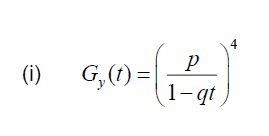
\( \left( \frac{p}{1 – q t} \right)^4 \)

\( Y = X_1 + X_2 + X_3 + X_4 \), independent

\( G_Y(t) = [G_X(t)]^4 \)



Result: \( \left( \frac{p}{1 – q t} \right)^4 \) [2]

(b)(ii)
\( 20 p^4 (1 – p)^3 \)

Method 1: Coefficient of \( t^3 \) in \( G_Y(t) = p^4 (1 – q t)^{-4} \)

\( (1 – q t)^{-4} = \sum_{k=0}^{\infty} \binom{k + 3}{k} q^k t^k \)

Coefficient of \( t^3 \): \( \binom{6}{3} q^3 = 20 q^3 \)

\( P(Y = 3) = p^4 \cdot 20 q^3 = 20 p^4 (1 – p)^3 \)

Method 2: \( P(Y = 3) = \frac{G_Y^{(3)}(0)}{3!} \)

\( G_Y^{(3)}(t) = 120 p^4 q^3 (1 – q t)^{-7} \)

At \( t = 0 \): \( G_Y^{(3)}(0) = 120 p^4 q^3 \)

\( P(Y = 3) = \frac{120 p^4 q^3}{6} = 20 p^4 q^3 = 20 p^4 (1 – p)^3 \)

Result: \( 20 p^4 (1 – p)^3 \) [2]