IB Mathematics AI AHL Walks, trails, paths, circuits, cycles MAI Study Notes - New Syllabus

IB Mathematics AI AHL Walks, trails, paths, circuits, cycles MAI Study Notes

LEARNING OBJECTIVE

Tree and cycle algorithms with undirected graphs. Walks, trails, paths, circuits, cycles

Key Concepts:

Walks
Chinese Postman Problem
Travelling Salesman Problem
Bounds for Travelling Salesman Problem

ROUTES ON THE GRAPH

Path: no vertex is revisited: e.g. ABC or AECD
Trail: no edge is revisited: e.g. AEBCED or BECBA
Walk: Walk as you wish, e.g. ABCBEC or ABAE

a path from X to Y looks like

a trail from X to Y looks like

Cycle: derived from a path which closes to the initial vertex e.g. ABEA or EBCDE (only the first vertex is revisited)
Circuit: a trail which closes to the initial vertex, e.g. AEDCEBA

(a walk which closes to the initial vertex is nothing more than a walk which closes to the initial vertex\! e.g. ABABABA)

The number of edges on a path, trail or walk is called length.

For example:

AB is a path of length 1 (just an edge)
ABC is a path of length 2.
AEBCED is a trail of length 5.
ABABABA is a walk of length 6 [one less than the number of vertices listed].

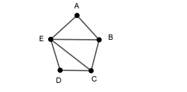
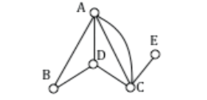
Example

For the given graph classify all the routes

▶️Answer/Explanation

Solution:

Sequence	Walk	Trail	Path	Circuit	Cycle
ADCFG	✓	✓	✓	✗	✗
CFEHFGC	✓	✓	✗	✓	✗
DCBEFCE	✓	✓	✗	✗	✗
ABEFGDA	✓	✓	✓	✓	✓
GCDCFC	✓	✗	✗	✗	✗

Eulerian Graphs

Eulerian Trail

A trail that uses every edge exactly once.
May start and end at different vertices.
Also known as a semi-Eulerian trail.

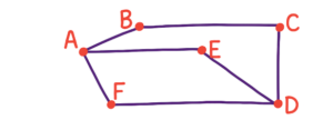
Example

Give an Eulerian trail for the following graph:

▶️Answer/Explanation

Solution:

ABCDEAFD is an Eulerian trail, using every edge, without repeating any.

Eulerian Circuit

A closed trail that uses every edge exactly once and returns to the starting vertex.
Also known as a Eulerian cycle.

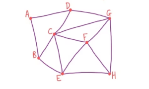
Example

Give an Eulerian circuit for the following graph:

▶️Answer/Explanation

Solution:

ADFAEDCBA is an Eulerian circuit.

Procedure to Classify a Graph

The graph is Eulerian if and only if all vertices have even degrees

The graph is semi-Eulerian if and only if all vertices, except two vertices X and Y, have even degrees.
The vertices X and Y have odd degrees (we call them odd vertices) and the trail has to start from X and finish at Y or vice versa

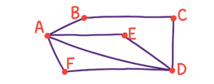
In the first graph(Semi-Eulerian Graph), only A and B have odd degrees (odd vertices). That is why the trail has to start from A and finish at B

In the second graph(Semi-Eulerian Graph) all vertices have even degrees.

Hamiltonian Paths and Cycles

Hamiltonian Cycle

A cycle that visits every vertex exactly once and returns to the starting vertex.
The graph is called Hamiltonian if such a cycle exists.

For the first one a Hamiltonian cycle is ABCEDA
For the second one a Hamiltonian cycle is ADECBFA

Hamiltonian Path

A path that visits every vertex exactly once but does not return to the starting vertex.
The graph has a Hamiltonian path even if it is not Hamiltonian (i.e., no cycle exists).

The graph is not Hamiltonian We can visit though all vertices by a path: ECBAD Such a path is called Hamiltonian path.

Properties

A Hamiltonian cycle in a graph with n vertices has length n.
Hamiltonian graphs may contain multiple Hamiltonian cycles and paths.

Example

Does a Hamiltonian path or circuit exist on the graph below?

▶️Answer/Explanation

Solution:

We can see that once we travel to vertex E there is no way to leave without returning to C, so there is no possibility of a Hamiltonian circuit. If we start at vertex E we can find several Hamiltonian paths, such as ECDAB and ECABD

Minimum Spanning Tree (MST)

A spanning tree is a subgraph that includes all vertices of the graph and is a tree (no cycles).
A minimum spanning tree (MST) is a spanning tree with the smallest possible total edge weight.
There can be more than one MST if multiple trees have the same total weight.
Applications include network design (e.g., computer networks, road networks).

Example

If a weighted graph has four spanning trees , How many MST will be there?

▶️Answer/Explanation

Solution:

The MST is the one with total weight = 9

Kruskal’s Algorithm

Kruskal’s algorithm builds the MST by choosing edges in order of increasing weight:

Sort all edges in ascending order of weight.
Select the smallest edge. Add it to the MST if it doesn’t form a cycle.
Repeat step 2 until the MST contains exactly n−1 edges (where n is the number of vertices).

Note:

Use a cycle-checking method like Union-Find (Disjoint Set).
If multiple edges have the same weight, choose any (randomly or by rule).

Example

Apply Kruskal’s algorithm on the following graph

▶️Answer/Explanation

Solution:

We have 5 vertices, we need $n-1 = 4$ edges

The minimum spanning tree is

It has total weight $28$.

Prim’s Algorithm

Prim’s algorithm builds the MST by growing a tree starting from an arbitrary vertex:

Start from any vertex.
Add the nearest vertex (with the smallest connecting edge) that is not already in the tree.
Repeat step 2 until all vertices are included.

Note:

Often implemented efficiently using a priority queue (min-heap).
Like Kruskal’s, if there’s a tie, choose any edge.

Example

Apply Prim’s algorithm on the following graph

▶️Answer/Explanation

Solution:

We have 5 vertices; we have to join all of them
Let us start from C. The tree now contains only C

The minimum spanning tree is as in example 1.
Total weight = $9+7+5+7 = 28$

Definition

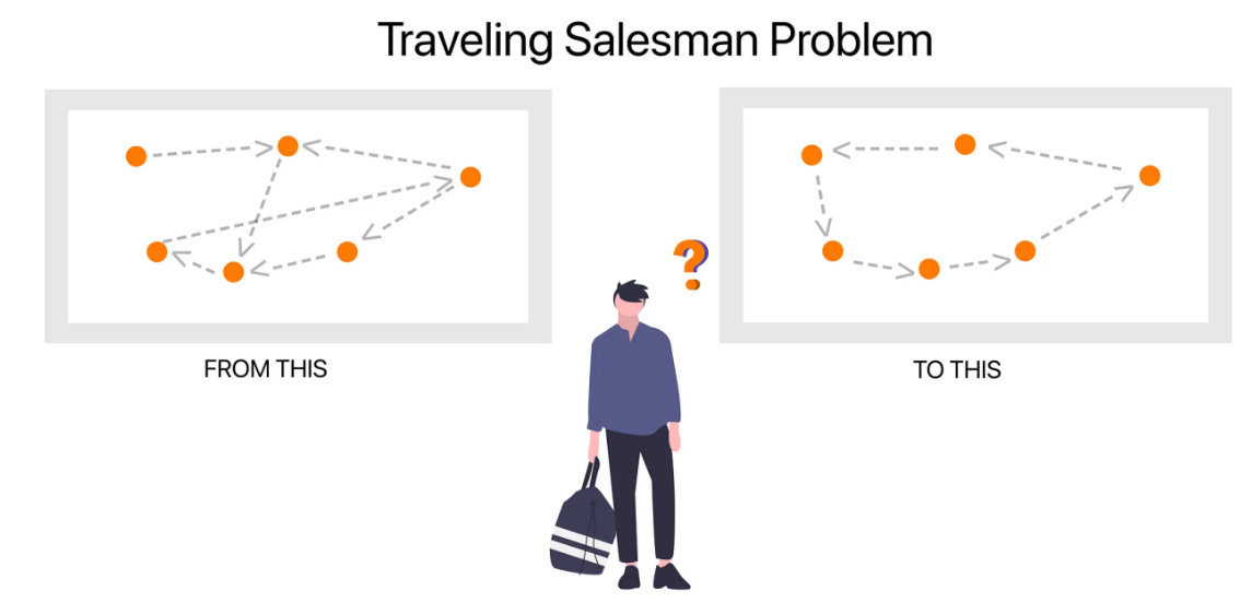
The Traveling Salesman Problem (TSP) is a classic optimization problem in graph theory. It asks:

“Given a list of cities and the distances between each pair of them, what is the shortest possible route that visits each city exactly once and returns to the starting city?”

Graph Structure

TSP can be modeled using a complete weighted graph where:

Each vertex represents a city.
Each edge represents a route between cities, weighted by distance, cost, or time.

Characteristics

It is a Hamiltonian cycle problem with optimization.
The number of possible routes grows factorially with the number of cities: $ (n-1)!/2 $ for undirected graphs.
It is an NP-hard problem — exact solutions are computationally expensive for large graphs.

Example:

Consider 4 cities: A, B, C, D. The distances between them are as follows:

Weighted Adjacency Table:

$\begin{array}{c|cccc} & A & B & C & D \\ \hline A & – & 10 & 15 & 20 \\ B & 10 & – & 35 & 25 \\ C & 15 & 35 & – & 30 \\ D & 20 & 25 & 30 & – \\ \end{array} $

what is the shortest possible route that visits each city exactly once and returns to the starting city?

▶️ Answer/Explanation

Solution:

One possible route: A → B → D → C → A

Total cost: $ 10 + 25 + 30 + 15 = 80 $

This problem tries all permutations of visiting cities once and returning to the start.
For 4 cities, there are $ \frac{(4-1)!}{2} = 3 $ unique Hamiltonian circuits to check (excluding symmetry).
The route with the lowest total cost is the solution to the TSP.
Heuristics like the nearest neighbor algorithm or minimum spanning tree-based approximation are used for larger graphs.

Common Methods to Solve TSP

Brute-force: Try all permutations (exact but inefficient for large $ n $).
Nearest Neighbor Heuristic: Always go to the nearest unvisited city.
Minimum Spanning Tree (MST) Approximation: Use MST to find a rough tour (e.g., Christofides’ algorithm).
Dynamic Programming: Held-Karp algorithm with time complexity $ O(n^2 \cdot 2^n) $.

Table of Least Weight – TSP

In the Traveling Salesman Problem, a Table of Least Weight is used to compare all possible Hamiltonian circuits and determine which route yields the minimum total weight (distance or cost).

This table is essential for solving small-scale TSP instances by listing:

Each possible route starting and ending at the same vertex.
The total weight of that route calculated by summing the edge weights.

Example:

Consider the following distances between cities:

$ \begin{array}{c|cccc} & A & B & C & D \\ \hline A & – & 10 & 15 & 20 \\ B & 10 & – & 35 & 25 \\ C & 15 & 35 & – & 30 \\ D & 20 & 25 & 30 & – \\ \end{array} $

Create table of least weight.

▶️ Answer/Explanation

Solution:

All Possible Circuits and Their Weights:

Route	Weight
A → B → C → D → A	10 + 35 + 30 + 20 = 95
A → B → D → C → A	10 + 25 + 30 + 15 = 80
A → C → B → D → A	15 + 35 + 25 + 20 = 95
A → C → D → B → A	15 + 30 + 25 + 10 = 80
A → D → B → C → A	20 + 25 + 35 + 15 = 95
A → D → C → B → A	20 + 30 + 35 + 10 = 95

Least Weight Routes: A → B → D → C → A or A → C → D → B → A

Total Cost: 80

All possible Hamiltonian circuits starting and ending at A are listed.
The total weights are computed by summing edge weights.
Among these, the minimal total cost is 80.
Either A → B → D → C → A or A → C → D → B → A are valid minimum-cost solutions.

Chinese Postman Problem

The goal is to find the shortest closed walk that traverses every edge at least once and returns to the starting point on a weighted graph (where):

Edges represent roads
Vertices represent junctions/crossroads
The postman wants to deliver mail by covering all roads with minimum total distance

Case 1: Eulerian Graph

All vertices have even degree.

A Eulerian circuit (a closed path visiting every edge exactly once).
Minimum cost = Total weight of all edges

Case 2: Semi-Eulerian Graph (2 Odd Vertices)

Exactly two vertices have odd degree (say, X and Y).

Find the shortest path from X to Y with weight a.

A Eulerian trail from X to Y
Plus a shortcut (duplicate) from Y to X along the shortest path
Minimum cost = Total weight + a

Case 3: 4 Odd Vertices (X, Y, Z, W)

Choose the best pairing of odd vertices such that the total added weight is minimized.

Compute shortest path weights:

X–Y and Z–W: weights a, b

X–Z and Y–W: weights c, d

X–W and Y–Z: weights e, f

Pick the pairing with the smallest total (e.g. a + b)
Add duplicate/fake edges for these two paths (X–Y and Z–W)
The graph becomes Eulerian
Find a Eulerian circuit, and when reaching X or Z, follow the duplicated path

Minimum cost = Total weight + (a + b)

Example

Solve the following Chinese postman problem.

▶️Answer/Explanation

Solution:

All vertices have even degree, so the graph is Eulerian.
Thus, the best solution has
total weight = (sum of weights) $= 45$
If we start from A, a possible route is $\rm{ABCDFEDBEA}$

Example

Solve the following Chinese postman problem.

▶️Answer/Explanation

Solution:

There are exactly two odd vertices: E (degree 3) and D (degree 3)
(so the graph is semi-Eulerian).
The shortest path from E to D is EBD of total weight 9.
Thus, the best solution has
$\text{total weight = (sum of weights) + 9 = 41 + 9 = 50}$
If we start from A, a possible route is $\rm{ABCDEBDBEA}$

Nearest Neighbor Algorithm (Upper Bound)

This algorithm builds a tour by always going to the nearest unvisited vertex.

Steps:

Start from any vertex.
Go to the nearest unvisited vertex.
Repeat step 2 until all vertices are visited.
Return to the starting vertex.

Result:

Gives a Hamiltonian cycle
Provides an upper bound on the minimum possible distance

Example:

Start at A
→ Closest vertex: B
→ Next closest: C
→ until all are visited
→ Return to A

Upper Bound = Total distance of this tour

Deleted Vertex Algorithm (Lower Bound)

This is a way to estimate the minimum possible length of a TSP tour — a lower bound, not an actual tour.

Steps:

Pick a vertex to delete (commonly the starting vertex).
Find a Minimum Spanning Tree (MST) on the remaining vertices.
Add the two smallest edges connecting the deleted vertex to the rest.
These simulate entering and exiting that vertex.
Lower Bound = Weight of MST + weight of 2 shortest connecting edges

Why this works:

Any valid Hamiltonian cycle must connect the deleted vertex to the rest of the graph at least twice, and contain at least an MST for the rest.
So this sum gives a minimum possible total.

Previous Topic Notes

Next Topic Notes

IB Mathematics AI AHL Walks, trails, paths, circuits, cycles MAI Study Notes - New Syllabus

IB Mathematics AI AHL Walks, trails, paths, circuits, cycles MAI Study Notes

ROUTES ON THE GRAPH

Minimum Spanning Tree (MST)

Traveling Salesman Problem (TSP)

Chinese Postman Problem

Resources

Members

Company