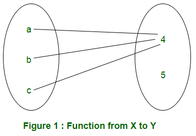
A function from a set $X$ to a set $Y$, written as:
$f: X \rightarrow Y$
assigns to each element $x \in X$ exactly one element $y \in Y$.
This relationship is written as:
$
\begin{aligned}
f(x) &= y \\
f : x &\mapsto y
\end{aligned}
$
We say that:
“$f$ maps $x$ to $y$” or “$y$ is the image of $x$ under $f$”
For example: $X = {a, b, c}$ and $Y = {4, 5}.$ A function from X to Y can be represented
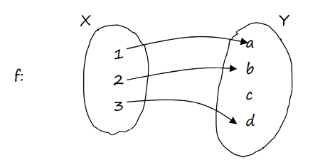
Example Let $X = \{1, 2, 3\}$ and $Y = \{a, b, c, d\}$. A relation $f: X \rightarrow Y$ is defined as follows: $f(1) = a$ Is this relation a function from $X$ to $Y$? Justify your answer.
▶️Answer/ExplanationSolution: Indeed, each element of \( X \) has a unique image in \( Y \). We write \( \begin{aligned} |
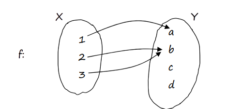
Example Let $X = \{1, 2, 3\}$ and $Y = \{a, b, c, d\}$. A relation $f: X \rightarrow Y$ is defined as follows: $f(1) = a$ Is this relation a function from $X$ to $Y$? Justify your answer.
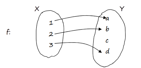
▶️Answer/ExplanationSolution: The following is a function(we do not mind if two elements of \( X \) have the same image) |
Note:
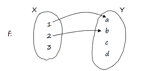
(we said “each \( x \) of \( X \),” but here 3 has no image) so this is not function.
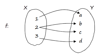
(we said “unique \( y \) of \( Y \),” but 2 has two images) for f(2) , so this is not function.
For a function \( f: X \rightarrow Y \),
The set of all \( x \)’s involved is called DOMAIN
The set of all \( y \)’s involved (only the images) is called RANGE
Consider again the function \( f: X \rightarrow Y \) given by
Then
DOMAIN: \( x \in X = \{1, 2, 3\} \)
RANGE: \( y \in \{a, b, d\} \)
We usually denote the domain by \( D_f \) and the range by \( R_f \).
GRAPH
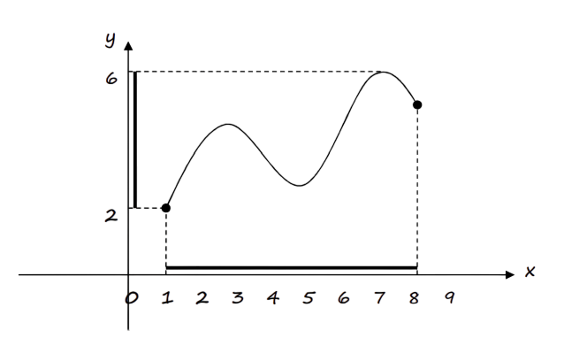
DOMAIN:
Projection on the \( x \)-axis, i.e. \( D_f: x \in [1, 8] \)
RANGE:
Projection on the \( y \)-axis, i.e. \( R_f: y \in [2, 6] \)
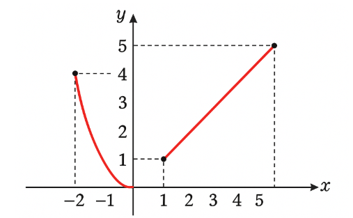
Example Consider the function \( f(x) = \begin{cases} x^2, & -2 \leq x \leq 0 \\ x, & 1 \leq x \leq 5 \end{cases} \) Sketch the graph. Also mention domain and range. ▶️Answer/ExplanationSolution:
$D_f : x \in [-2, 0] \cup [1, 5] \quad \text{and} \quad R_f : y \in [0, 5]$ |
NOTE:
The graph also shows if we have a function or not
This is not a function, since \( f(3) \) for example is not unique!
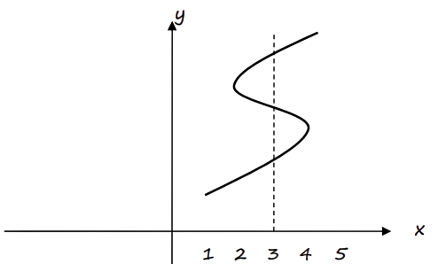
Vertical line test:
Any vertical line intersects the graph at most once.
AN “AGREEMENT” FOR THE DOMAIN
Usually, a function is simply given as a formula of the form \( y = f(x) \), where \( x \) and \( y \) are real variables.
If the domain of the function is not given, we agree that
\( D_f \text{ is } \mathbb{R} \)
or \( D_f \) is the largest possible subset of \( \mathbb{R} \)
For example,
if \( f \) is given by \( f(x) = 2x \), we assume that \( x \in \mathbb{R} \)
if \( f \) is given by \( f(x) = \frac{2}{x} \), we assume that \( x \in \mathbb{R} – \{0\} = \mathbb{R} \)
(we may also write \( D_f: x \neq 0 \))
1. \( f(x) \) is a function with no restrictions on \( x \),
for example a polynomial [say \( f(x) = 2x^3 + 3x^2 + 1 \)], then
\( D_f = \mathbb{R} \)
2. \( f(x) = \frac{A}{B} \), then \( B \) cannot be 0, thus
\( D_f = \mathbb{R} – \{\text{roots of the equation } B = 0\} \)
3. \( f(x) = \sqrt{A} \), then \( A \geq 0 \).
\( D_f = \text{the solution set of the inequality } A \geq 0 \)
4. \( f(x) = \log A \) or \( f(x) = \ln A \), then \( A > 0 \).¹
\( D_f = \text{the solution set of the inequality } A > 0 \)
Example Find Domain of following a) \( f(x) = 3x – 9 \) b) \( f(x) = \dfrac{5}{3x – 9} \) c) \( f(x) = \sqrt{3x – 9} \) d) \( f(x) = \ln(3x – 9) \) e) \( f(x) = \dfrac{x + 2}{x^2 – 3x + 2} \) f) \( f(x) = \sqrt{x – 1} + \sqrt[3]{2 – x} \) g) \( f(x) = \dfrac{\sqrt{1 – x^2}}{x} \) ▶️Answer/ExplanationSolution: a) $D_f : x \in \mathbb{R}$ b) $D_f : x \in \mathbb{R} \setminus \{3\} \quad$ or $\quad D_f : x \neq 3$ c) $D_f : x \in [3, +\infty) \quad$ or $\quad D_f : x \geq 3$ d) $D_f : x \in (3, +\infty) \quad$ or $\quad D_f : x > 3$ e) $D_f : x \in \mathbb{R} \setminus \{1, 2\}$ f) $D_f : x \in [1, 2] \quad$ or $\quad D_f : 1 \leq x \leq 2$ g) $D_f : x \in [-1, 0) \cup (0, 1]$ |
The inverse function of \( f \), that is \( g \), will be denoted by \( f^{-1} \)
\( \begin{aligned}
f(x) &= x + 10 \\
f^{-1}(x) &= x – 10
\end{aligned} \)
Mathematically
\( \text{If } f(x) = y \text{ then } f^{-1}(y) = x . \)
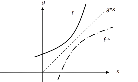
In fact, \( f \) and \( f^{-1} \) are inverse to each other.
The graph of \( f^{-1} \) is a reflection of \( f \) about the line \( y = x \)
|
Example If \( f(x) = x^2 \), for \( x \geq 0 \), then \( f^{-1}(x) = \sqrt{x} \). Discuss it true or not? ▶️Answer/ExplanationSolution: \( f \) and \( f^{-1} \) intersect on the line \( y = x \). |
THE INVERSE FUNCTION IN REAL LIFE PROBLEMS
In real life problems instead of \( x \) and \( y \) we may have other parameters.
For example, a square of side \( a \) has
Perimeter \( P = 4a \)
Area \( A = a^2 \)
(it is the function \( y = 4x \))
(it is the function \( y = x^2 \))
If they give us the perimeter \( P \), then
\( P = 4a \Leftrightarrow a = \frac{P}{4} \)
Now the side is given in terms of the perimeter. This is in fact the inverse function of \( P = 4a \)
If they give us the area \( A \), then
\( A = a^2 \Leftrightarrow a = \sqrt{A} \)
Now the side is given in terms of the area. This is in fact the inverse function of \( A = a^2 \).
|
Example Let \( F \) denote the temperature in Fahrenheit degrees & \( C \) denote the temperature in Celsius degrees The conversion from Celsius to Fahrenheit is given by \( F = 1.8C + 32 \) \( F(30) = 86 \) implies that \( 30^\circ \) Celsius is equal to \( 86^\circ \) Fahrenheit ▶️Answer/ExplanationSolution: If we solve for \( C \) then \( C = \frac{F – 32}{1.8} \) \( C(86) = 30 \) implies that \( 86^\circ \) Fahrenheit is equal to \( 30^\circ \) Celsius We can say that \( \begin{aligned} |