A linear model represents a relationship between two variables where the rate of change is constant. The graph is a straight line, and the model is used when changes in one quantity result in proportional changes in another.

Form:
$y = mx + c$
$m$: Slope (rate of change)
$c$: y-intercept
Usage:
Constant rate of change.
Example:
A taxi charges \$3 base fare and \$2 per km.
$\text{Cost} = 2x + 3$
Example: A taxi company charges a flat fee of \$3 plus \$2 per kilometer. Find the cost of a 10 km ride. ▶️Answer/ExplanationSolution: $ \text{Cost} = 2x + 3 $ $ x = 10 \Rightarrow \text{Cost} = 2(10) + 3 = 20 + 3 = \boxed{23} $ |
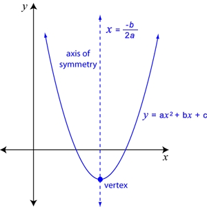
A quadratic model describes a relationship where the rate of change itself changes at a constant rate. The graph is a parabola that opens upwards or downwards. It’s often used to model situations involving acceleration or area.
Form:
$y = ax^2 + bx + c$
Parabola shape
Vertex: $x = -\frac{b}{2a}$
Usage:
Projectile motion, area problems, acceleration.
Example:
Height $h$ of a ball thrown upward:
$h(t) = -4.9t^2 + 20t + 1.5$
By GDC:
TI-nspire $\implies$ MENU $\implies$ 6: ANALYZE GRAPH
$\implies$ 1: ZERO $\implies$ Choose lower & upper bound
$\implies$ ENTER $\implies$ Root given
TI-84 $\implies$ 2nd CALC $\implies$ 2: ZERO
$\implies$ Choose left & right bound
$\implies$ ENTER ENTER
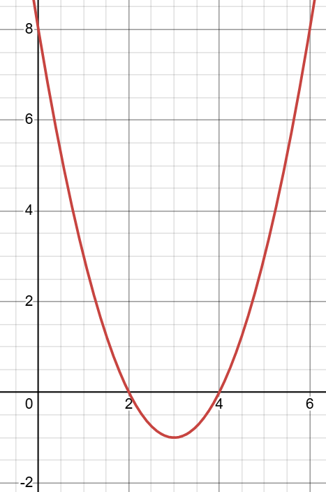
Example: Find y-intercept , Axis of symmetry ,Vertex , Roots (by factoring) of $f(x) = x^2 – 6x + 8$: Sketch the graph using GDC ▶️Answer/ExplanationSolution: y-intercept: $ Axis of symmetry: $ Vertex: $ Roots (by factoring): $
|
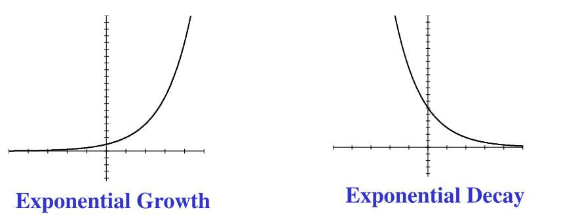
Exponential models show situations where quantities grow or decrease at rates proportional to their current value. These models are used for population growth, radioactive decay, interest, and more.
Form:
Growth: $y = a(1 + r)^t$
Decay: $y = a(1 – r)^t$
or
General: $y = ab^x$
Where:
$a$: initial amount
$r$: growth/decay rate
$t$: time
$b > 1$ for growth, $0 < b < 1$ for decay
Example (growth): Population doubles every 5 years:
$P(t) = 500 \cdot 2^{t/5}$
Example: A population of bacteria doubles every 3 hours. Initial population: 500. Model: $ P(t) = 500 \cdot 2^{t/3} $ What is the population after 6 hours? ▶️Answer/ExplanationSolution: $ P(6) = 500 \cdot 2^{6/3} = 500 \cdot 2^2 = 500 \cdot 4 = \boxed{2000} $ |
Direct Variation –
A direct variation describes a linear relationship where one variable is a constant multiple of another (i.e., they increase or decrease together at the same ratio).
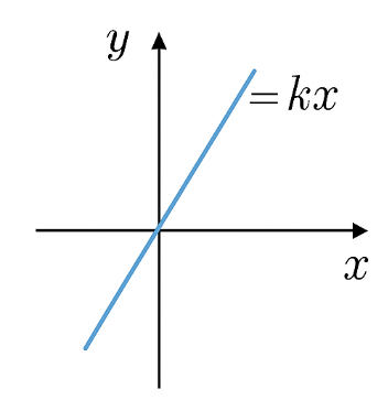
Form:
$y = kx$
$k$: constant of proportionality
Example:
If $y$ varies directly with $x$ and $y = 10$ when $x = 2$, then:
$k = \frac{y}{x} = 5 \Rightarrow y = 5x$
Inverse Variation –
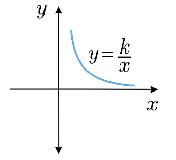
An inverse variation describes a relationship where the product of two variables is constant. As one increases, the other decreases proportionally.
Form:
$y = \frac{k}{x}$
Example:
If $y$ varies inversely with $x$ and $y = 4$ when $x = 3$:
$k = yx = 12 \Rightarrow y = \frac{12}{x}$
(a) Direct Variation) Example: $y \propto x$, and $y = 12$ when $x = 4$. Find: $y$ when $x = 6$ ▶️Answer/ExplanationSolution: $ y = kx \Rightarrow 12 = k(4) \Rightarrow k = 3 $ $ y = 3x \Rightarrow y = 3(6) = \boxed{18} $ (b) Inverse Variation) Example: $y \propto \frac{1}{x}$, and $y = 5$ when $x = 2$. Find: $y$ when $x = 10$ ▶️Answer/ExplanationSolution: $ y = \frac{k}{x} \Rightarrow 5 = \frac{k}{2} \Rightarrow k = 10 $ $ y = \frac{10}{10} = \boxed{1} $ |
A cubic model represents relationships involving three-degree polynomials. The graph can have one or two turning points and is used to model more complex growth patterns or changes in direction.
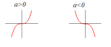
Form:
$y = ax^3 + bx^2 + cx + d$
Can have up to 3 real roots and 2 turning points
Usage:
Non-linear motion, volume growth, economics.
Example:
$y = x^3 – 6x^2 + 11x – 6$
Example: A function is defined by $ f(x) = x^3 – 3x^2 + 2x $ Find $f(2)$ ▶️Answer/ExplanationSolution: $ f(2) = (2)^3 – 3(2)^2 + 2(2) = 8 – 12 + 4 = \boxed{0} $ |
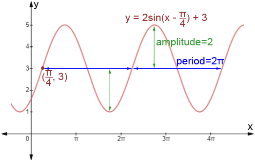
Sinusoidal models use sine or cosine functions to represent periodic phenomena that repeat at regular intervals, such as seasonal temperatures, sound waves, or tides.
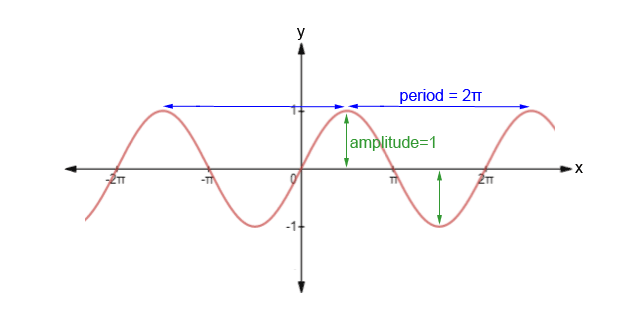
Form:
$y = a \sin(bx + c) + d \quad \text{or} \quad y = a \cos(bx + c) + d$
Where:
$a$: amplitude
$b$: affects period $= \frac{2\pi}{|b|}$
$c$: phase shift
$d$: vertical shift
Usage:
Seasonal data, waves, pendulum motion.
Example: Temperature variation during a day
$T(t) = 10 \cos\left(\frac{\pi}{12}t – \frac{\pi}{2}\right) + 20$
Example: Describe the key characteristics and transformations of the graph of the function $y = 2\sin(x – \frac{\pi}{4}) + 3$. ▶️Answer/ExplanationSolution: Graph $y = 2\sin(x – \frac{\pi}{4}) + 3$. Period: $\frac{2\pi}{B} = \frac{2\pi}{1} = 2\pi$
|