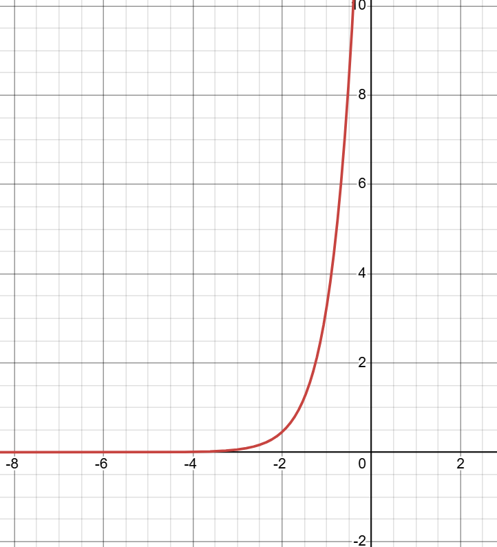
Exponential models are commonly used in Math AI to repre=sent real-world situations involving consistent rates of growth or decay over time.
A common application of exponential models is in modeling *population growth*, which is useful in environmental science, economics, and epidemiology.
The general form of an exponential model is:
\( f(x) = a \cdot b^x \)
where:
\( a \) is the initial value
\( b \) is the base (often \( e \) for natural exponential functions)
\( x \) is the independent variable (typically time)
Decay Models and Half-Life
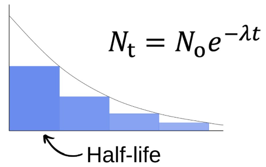
For modeling decay, especially with half-life problems, we often use:
\( N(t) = N_0 \cdot e^{-\lambda t} \)
where:
\( N(t) \) is the quantity at time \( t \)
\( N_0 \) is the initial quantity
\( \lambda \) is the decay constant
\( t \) is the time elapsed
Example Suppose a certain medication degrades in the body with a half-life of 4 hours. If a patient starts with 200 mg of the drug, the amount left at time \( t \) can be modeled by: \( N(t) = 200 \cdot e^{-(\ln 2 / 4) \cdot t} \) Find the amount remaining after 10 hours: ▶️Answer/ExplanationSolution: \( N(10) = 200 \cdot e^{-(\ln 2 / 4) \cdot 10} \approx 35.36 \text{ mg} \) |
Sinusoidal models are used to describe periodic phenomena, such as sound waves, alternating current, and seasonal temperature variations. The general form is:
$ f(x) = a \sin(b(x – c)) + d $
where:
\(a\) is the amplitude (half the distance between the maximum and minimum values).
\(b\) affects the period (which is \( \frac{2\pi}{b} \) in radians).
\(c\) is the phase shift (horizontal translation).
\(d\) is the vertical shift (midline of the oscillation).
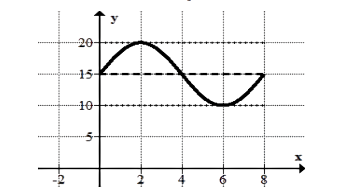
Example The graph of $f(x) = A\sin(Bx^\circ) + C$ is given below. Find A, B, C.
▶️Answer/ExplanationSolution: The curve is of type +sinx (since y-int central/up) Central axis at $y = 15$, so $C = 15$ Therefore, the equation of the function is $ |
The function of this model (called logistic) has the form
$ f(x) = \frac{L}{1 + Ce^{-kx}} $
The three parameters \( L, C, k \) are all positive.
Consider for example the function
$ y = \frac{100}{1 + 4e^{-2x}} $
Look at the graph of this function on your GDC with V-window:
\( -5 < x < 5 \) and \( -20 < y < 70 \)
It looks like exponential. But it is not! If we increase the upper bound for \( y \), we will realise that the behaviour of the graph changes dramatically.
After a while, this S-shape curve tends to be constant. In fact, it has a horizontal asymptote at \( y = 100 \).
This function is called logistic, and it is the model in many real-life situations.
The spread of a virus on Earth is usually exponential in early stages. Theoretically, it tends to \( +\infty \) as time goes by. However, the population on Earth is not infinite, so there is an upper limit for this spread.
The graph of a logistic model
$ y = \frac{L}{1 + Ce^{-kx}} $
looks like:
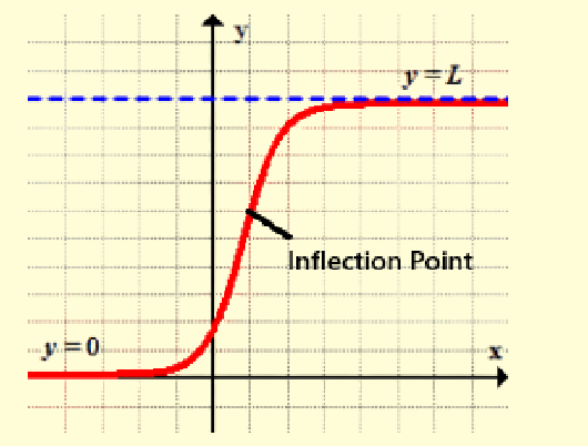
Horizontal asymptote:
\( y = L \)
\( y \)-intercept: \( y = \frac{L}{1 + C} \) (when \( x = 0 \))
The parameter \( k \) determines the growth rate or steepness of the curve.
In our example:
$ y = \frac{100}{1 + 4e^{-2x}} $
The horizontal asymptote is
\( y = 100 \).
Indeed, as \( x \to +\infty \), \( e^{-2x} \to 0 \), so \( y \to 100 \).
The \( y \)-intercept (for \( x = 0 \)) is \( y = \frac{100}{1 + 4} = 20 \).
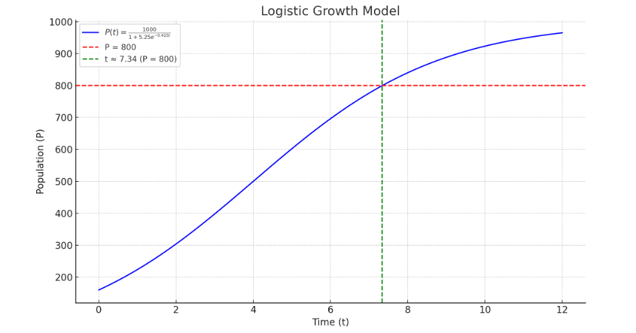
Example The logistic model \( P = \frac{L}{1 + Ce^{-kt}} \) It has a limiting value \( P = 1000 \). Using the logistic model find all the parameters Sketch the graph , motion both the asymptotes. ▶️Answer/ExplanationSolution: We also know the data: Clearly, \( L = 1000 \). For \( t = 0 \), \( P = 160 \): $ \frac{L}{1 + C} = 160 \Rightarrow \frac{1000}{1 + C} = 160 \Rightarrow 1 + C = 6.25 \Rightarrow C = 5.25 $ For \( t = 4 \), \( P = 500 \): $ \frac{1000}{1 + 5.25e^{-4k}} = 500 \Rightarrow \frac{1000}{500} = 1 + 5.25e^{-4k} \Rightarrow 5.25e^{-4k} = 1 $ $ \Rightarrow e^{4k} = 5.25 \Rightarrow 4k = \ln 5.25 \Rightarrow k = \frac{\ln 5.25}{4} \approx 0.415 $ Therefore, $ P = \frac{1000}{1 + 5.25e^{-0.415t}} $ The value of \( P \) exceeds 800 when \( t = 7.34 \) (use GDC to confirm).
|
A piecewise function has different expressions in different intervals. For example,
$ f(x) =
\begin{cases}
-x + 6, & 0 \leq x < 2 \\
x^2, & 2 \leq x < 4 \\
256 \times 2^{-x}, & 4 \leq x \leq 10
\end{cases} $
which is linear in the \(1^{st}\) interval, quadratic in the \(2^{nd}\) interval and exponential in the \(3^{rd}\) interval.
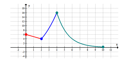
Usually, we require such a function to be continuous, that is the right endpoint of each interval coincides with the left endpoint of the next interval.
For example, for the function above:
At \(x=2\): \(-x+6\) gives 4 \(x^2\) also gives 4
At \(x=4\): \(x^2\) gives 16 \(256 \times 2^{-x}\) also gives 16
Indeed, the curve of the function seems to be “continuous”:
Therefore, given some data with a different behaviour in different intervals we can construct a piecewise model function to describe this varying behavior.
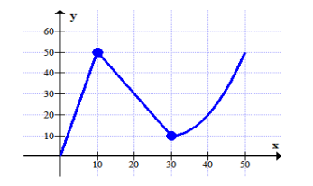
Example Peter investigated a series of data \((x,y)\) and observed that: between \(x=0\) and \(x=10\), \(y\) is proportional to \(x\) i.e. data follow a model of the form \(ax\) between \(x=10\) and \(x=30\), \(y\) decreases linearly in rate 2 i.e. data follow a model of the form \(-2x+b\) between \(x=30\) and \(x=50\), data follow the quadratic model \(0.1(x-30)^2 + 10\), (a) Write down a piecewise function \(f(x)\) that describes the data. ▶️Answer/ExplanationSolution: $ f(x) = (b) At \(x=10\): \(ax = -2x + b \implies 10a = -20 + b\) The solution of the system is \(b = 70\) and \(a = 5\). Thus, \(f(x)\) takes the form: $ f(x) = (c)
|