Linear Differential Equations of Type \( \displaystyle \frac{dy}{dx} + P(x)y = Q(x) \)
A linear differential equation is an equation in which the dependent variable \( y \) and its derivative \( \dfrac{dy}{dx} \) appear only to the first power and are not multiplied together.
The standard form is: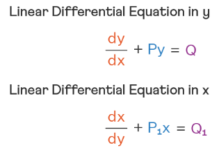
$ \dfrac{dy}{dx} + P(x)y = Q(x) $
Here,
- \( P(x) \) and \( Q(x) \) are known functions of \( x \).
- \( y \) is the dependent variable.
Standard Form and Integrating Factor (I.F.)
The equation is said to be in standard form if it can be written as:
$ \dfrac{dy}{dx} + P(x)y = Q(x) $
The Integrating Factor (I.F.)</strong) is defined as:
$ \text{I.F.} = e^{\int P(x)\,dx} $
General Solution
Multiplying both sides of the differential equation by the integrating factor:
$ e^{\int P(x)\,dx} \dfrac{dy}{dx} + e^{\int P(x)\,dx} P(x)y = Q(x)e^{\int P(x)\,dx} $
The left-hand side becomes the derivative of \( y \times \text{I.F.} \):
$ \dfrac{d}{dx}\left[y \cdot e^{\int P(x)\,dx}\right] = Q(x)e^{\int P(x)\,dx} $
Integrating both sides:
$ y \cdot e^{\int P(x)\,dx} = \int Q(x)e^{\int P(x)\,dx}\,dx + C $
Hence, the general solution is:
$ \boxed{y = e^{-\int P(x)\,dx}\left[\int Q(x)e^{\int P(x)\,dx}\,dx + C\right]} $
Steps to Solve
- Write the equation in standard form \( \dfrac{dy}{dx} + P(x)y = Q(x) \).
- Find the integrating factor \( \text{I.F.} = e^{\int P(x)\,dx} \).
- Multiply the entire equation by the I.F.
- Recognize that LHS = \( \dfrac{d}{dx}(y \cdot \text{I.F.}) \).
- Integrate both sides and solve for \( y \).
Special Case — When \( Q(x) = 0 \)
The equation reduces to:
$ \dfrac{dy}{dx} + P(x)y = 0 $
This is a homogeneous linear differential equation whose solution is:
$ y = Ce^{-\int P(x)\,dx} $
Example
Solve \( \dfrac{dy}{dx} + y = e^{-x} \).
▶️ Answer / Explanation
Step 1: Compare with standard form \( \dfrac{dy}{dx} + P(x)y = Q(x) \).
Here, \( P(x) = 1, \, Q(x) = e^{-x}. \)
Step 2: Find the integrating factor:
\( \text{I.F.} = e^{\int 1\,dx} = e^x. \)
Step 3: Multiply throughout by \( e^x \):
\( e^x\dfrac{dy}{dx} + e^x y = 1. \)
LHS = \( \dfrac{d}{dx}(y e^x) \). Hence,
\( \dfrac{d}{dx}(y e^x) = 1. \)
Step 4: Integrate both sides:
\( y e^x = x + C. \)
Step 5: Final Solution:
\( \boxed{y = e^{-x}(x + C).} \)
Example
Solve \( \dfrac{dy}{dx} + 2y = 4x \).
▶️ Answer / Explanation
Step 1: Standard form → \( P(x) = 2, \, Q(x) = 4x. \)
Step 2: Integrating Factor:
\( \text{I.F.} = e^{\int 2\,dx} = e^{2x}. \)
Step 3: Multiply the whole equation by \( e^{2x} \):
\( e^{2x}\dfrac{dy}{dx} + 2ye^{2x} = 4xe^{2x}. \)
LHS = \( \dfrac{d}{dx}(y e^{2x}) \). So,
\( \dfrac{d}{dx}(y e^{2x}) = 4xe^{2x}. \)
Step 4: Integrate both sides:
\( y e^{2x} = \int 4xe^{2x}\,dx. \)
Using integration by parts: \( \int xe^{2x}\,dx = \dfrac{xe^{2x}}{2} – \dfrac{e^{2x}}{4}. \)
\( \Rightarrow y e^{2x} = 4\left(\dfrac{xe^{2x}}{2} – \dfrac{e^{2x}}{4}\right) + C = 2xe^{2x} – e^{2x} + C. \)
Step 5: Divide by \( e^{2x} \):
\( \boxed{y = 2x – 1 + Ce^{-2x}.} \)
Example
Solve \( \dfrac{dy}{dx} + \dfrac{y}{x} = \sin x \), for \( x > 0 \).
▶️ Answer / Explanation
Step 1: Standard form: \( P(x) = \dfrac{1}{x}, \, Q(x) = \sin x. \)
Step 2: Integrating Factor:
\( \text{I.F.} = e^{\int 1/x\,dx} = e^{\ln x} = x. \)
Step 3: Multiply through by \( x \):
\( x\dfrac{dy}{dx} + y = x\sin x. \)
LHS = \( \dfrac{d}{dx}(xy). \)
\( \dfrac{d}{dx}(xy) = x\sin x. \)
Step 4: Integrate both sides:
\( xy = \int x\sin x\,dx. \)
Integration by parts: \( \int x\sin x\,dx = -x\cos x + \sin x. \)
\( \Rightarrow xy = -x\cos x + \sin x + C. \)
Step 5: Final Solution:
\( \boxed{y = -\cos x + \dfrac{\sin x}{x} + \dfrac{C}{x}.} \)