Question
The following table shows the data collected from an experiment.
x | 3.3 | 6.9 | 11.9 | 13.4 | 17.8 | 19.6 | 21.8 | 25.3 |
y | 6.3 | 8.1 | 8.4 | 11.6 | 10.3 | 12.9 | 13.1 | 17.3 |
The data is also represented on the following scatter diagram.
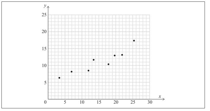
The relationship between x and y can be modelled by the regression line of y on x with equation y = ax + b , where a, b ∈ R.
Write down the value of a and the value of b . [2]
Use this model to predict the value of y when x = 18 . [2]
Write down the value of \(\bar{x}\) and the value of \(\bar{y}\) . [1]
Draw the line of best fit on the scatter diagram. [2]
▶️Answer/Explanation
Ans:
(a)
a = 0.433156…, b= 4.50265…
a = 0.433, b = 4.50
(b)
attempt to substitute x= 18 into their equation
y = 0.433 × 18 + 4.50
= 12.2994…
=12.3
(c) \(\bar{x}\)= 15 \(\bar{y}\) = 11
(d) 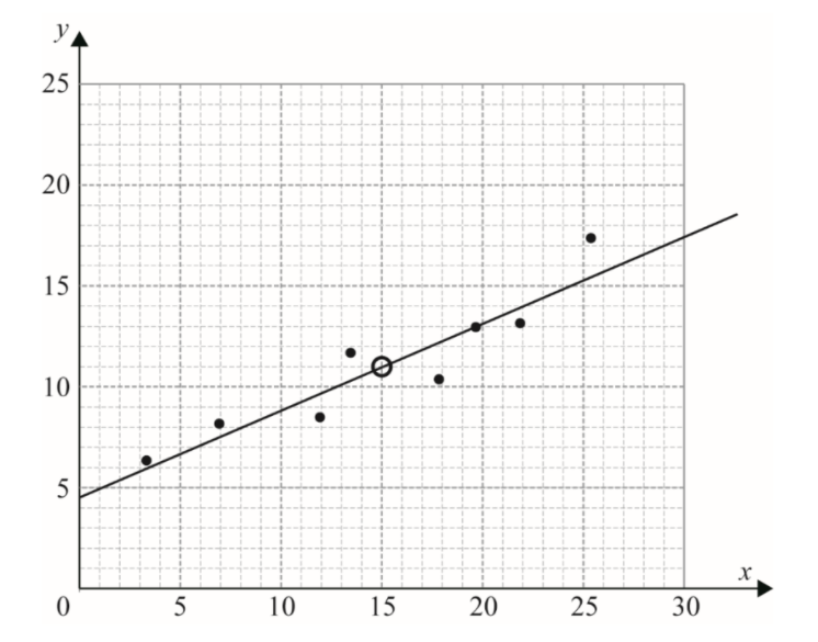
Question
At a café, the waiting time between ordering and receiving a cup of coffee is dependent upon the number of customers who have already ordered their coffee and are waiting to receive it. Filicia, a regular customer, visited the café on five consecutive days. The following table shows the number of customers, x , ahead of Filicia who have already ordered and are waiting to receive their coffee and Filicia’s waiting time, y minutes.
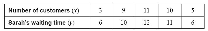
The relationship between x and y can be modelled by the regression line of y on x with equation y = ax + b .
(a) (i) Find the value of a and the value of b
(ii) Write down the value of Pearson’s product-moment correlation coefficient, r . [3]
(b) Interpret, in context, the value of a found in part (a)(i). [1]
On another day, Filicia visits the café to order a coffee. Seven customers have already ordered their coffee and are waiting to receive it.
(c) Use the result from part (a)(i) to estimate Filicia’s waiting time to receive her coffee. [2]
▶️Answer/Explanation
Ans:
(a)(i) From graphing calculator, we have $y=0.805x+2.88$, i.e., $a=0.805$ and $b=2.88$.
(a)(ii) Again, from graphing calculator, $r=0.978$.
(b) For each increase in customer ($x$), the corresponding waiting time ($y$) increases by $a=0.805$ minutes.
(c) When $x=7$, we have $y=8.52$, thus, Filicia has to wait for $8.52$ minutes to receive her coffee.
Question
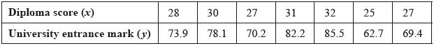
The following table shows the Diploma score \(x\) and university entrance mark \(y\) for seven IB Diploma students.
a.Find the correlation coefficient.[2]
The relationship can be modelled by the regression line with equation \(y = ax + b\).
b.Write down the value of \(a\) and of \(b\).[2]
c.Rita scored a total of \(26\) in her IB Diploma.
Use your regression line to estimate Rita’s university entrance mark.[2]
▶️Answer/Explanation
Markscheme
evidence of set up (M1)
eg\(\;\;\;\)correct value for \(r\) (or for \(a\) or \(r\), seen in (b))
\(0.996010\)
\(r = 0.996\;\;\;[0.996,{\text{ }}0.997]\) A1 N2
[2 marks]
\(a = 3.15037,{\text{ }}b = – 15.4393\)
\(a = 3.15{\text{ }}[3.15,{\text{ }}3.16],{\text{ }}b = – 15.4{\text{ }}[ – 15.5,{\text{ }} – 15.4]\) A1A1 N2
[2 marks]
substituting \(26\) into their equation (M1)
eg\(\;\;\;\)\(y = 3.15(26) – 15.4\)
\(66.4704\)
\(66.5{\text{ }}[66.4,{\text{ }}66.5]\) A1 N2
[2 marks]
Total [6 marks]
Question
The following table shows the sales, \(y\) millions of dollars, of a company, \(x\) years after it opened.
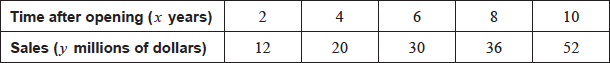
The relationship between the variables is modelled by the regression line with equation \(y = ax + b\).
a.(i) Find the value of \(a\) and of \(b\).
(ii) Write down the value of \(r\).[4]
b.Hence estimate the sales in millions of dollars after seven years.[2]
▶️Answer/Explanation
Markscheme
(i) evidence of set up (M1)
eg\(\;\;\;\)correct value for \(a\), \(b\) or \(r\)
\(a = 4.8,{\text{ }}b = 1.2\) A1A1 N3
(ii) \(r = 0.988064\)
\(r = 0.988\) A1 N1
[4 marks]
correct substitution into their regression equation (A1)
eg\(\;\;\;4.8 \times 7 + 1.2\)
\(34.8\) (millions of dollars) (accept \(35\) and \({\text{34}}\,{\text{800}}\,{\text{000}}\)) A1 N2
[2 marks]
Total [6 marks]
Question
An environmental group records the numbers of coyotes and foxes in a wildlife reserve after \(t\) years, starting on 1 January 1995.
Let \(c\) be the number of coyotes in the reserve after \(t\) years. The following table shows the number of coyotes after \(t\) years.
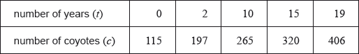
The relationship between the variables can be modelled by the regression equation \(c = at + b\).
a.Find the value of \(a\) and of \(b\).[3]
Use the regression equation to estimate the number of coyotes in the reserve when \(t = 7\).[3]
c.Find the number of foxes in the reserve on 1 January 1995.[3]
d.After five years, there were 64 foxes in the reserve. Find \(k\).[3]
e.During which year were the number of coyotes the same as the number of foxes?[4]
▶️Answer/Explanation
Markscheme
evidence of setup (M1)
eg\(\;\;\;\)correct value for \(a\) or \(b\)
\(13.3823\), \(137.482\)
\(a{\rm{ }} = {\rm{ }}13.4\), \(b{\rm{ }} = {\rm{ }}137\) A1A1 N3
[3 marks]
correct substitution into their regression equation
eg\(\;\;\;13.3823 \times 7 + 137.482\) (A1)
correct calculation
\(231.158\) (A1)
\(231\) (coyotes) (must be an integer) A1 N2
[3 marks]
recognizing \(t = 0\) (M1)
eg\(\;\;\;f(0)\)
correct substitution into the model
eg\(\;\;\;\frac{{2000}}{{1 + 99{{\text{e}}^{ – k(0)}}}},{\text{ }}\frac{{2000}}{{100}}\) (A1)
\(20\) (foxes) A1 N2
[3 marks]
recognizing \((5,{\text{ }}64)\) satisfies the equation (M1)
eg\(\;\;\;f(5) = 64\)
correct substitution into the model
eg\(\;\;\;64 = \frac{{2000}}{{1 + 99{{\text{e}}^{ – k(5)}}}},{\text{ }}64(1 + 99\(e\)^{ – 5k}}) = 2000\) (A1)
\(0.237124\)
\(k = – \frac{1}{5}\ln \left( {\frac{{11}}{{36}}} \right){\text{ (exact), }}0.237{\text{ }}[0.237,{\text{ }}0.238]\) A1 N2
[3 marks]
valid approach (M1)
eg\(\;\;\;c = f\), sketch of graphs
correct working (A1)
eg\(\;\;\;\frac{{2000}}{{1 + 99{{\text{e}}^{ – 0.237124t}}}} = 13.382t + 137.482\), sketch of graphs, table of values
\(t = 12.0403\) (A1)
\(2007\) A1 N2
Note: Exception to the FT rule. Award A1FT on their value of \(t\).
[4 marks]
Total [16 marks]
Question
Adam is a beekeeper who collected data about monthly honey production in his bee hives. The data for six of his hives is shown in the following table.
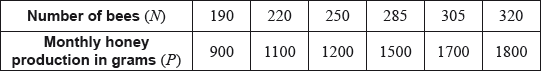
The relationship between the variables is modelled by the regression line with equation \(P = aN + b\).
Adam has 200 hives in total. He collects data on the monthly honey production of all the hives. This data is shown in the following cumulative frequency graph.
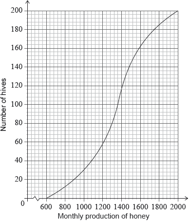
Adam’s hives are labelled as low, regular or high production, as defined in the following table.
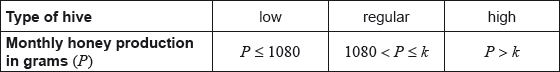
Adam knows that 128 of his hives have a regular production.
a.Write down the value of \(a\) and of \(b\).[3]
b.Use this regression line to estimate the monthly honey production from a hive that has 270 bees.[2]
c.Write down the number of low production hives.[1]
d.i.Find the value of \(k\);[3]
d.ii.Find the number of hives that have a high production.[2]
e.Adam decides to increase the number of bees in each low production hive. Research suggests that there is a probability of 0.75 that a low production hive becomes a regular production hive. Calculate the probability that 30 low production hives become regular production hives.[3]
▶️Answer/Explanation
Markscheme
evidence of setup (M1)
eg\(\,\,\,\,\,\)correct value for \(a\) or \(b\)
\(a = 6.96103,{\text{ }}b = – 454.805\)
\(a = 6.96,{\text{ }}b = – 455{\text{ (accept }}6.96x – 455)\) A1A1 N3
[3 marks]
substituting \(N = 270\) into their equation (M1)
eg\(\,\,\,\,\,\)\(6.96(270) – 455\)
1424.67
\(P = 1420{\text{ (g)}}\) A1 N2
[2 marks]
40 (hives) A1 N1
[1 mark]
valid approach (M1)
eg\(\,\,\,\,\,\)\(128 + 40\)
168 hives have a production less than \(k\) (A1)
\(k = 1640\) A1 N3
[3 marks]
valid approach (M1)
eg\(\,\,\,\,\,\)\(200 – 168\)
32 (hives) A1 N2
[2 marks]
recognize binomial distribution (seen anywhere) (M1)
eg\(\,\,\,\,\,\)\(X \sim {\text{B}}(n,{\text{ }}p),{\text{ }}\left( {\begin{array}{*{20}{c}} n \\ r \end{array}} \right){p^r}{(1 – p)^{n – r}}\)
correct values (A1)
eg\(\,\,\,\,\,\)\(n = 40\) (check FT) and \(p = 0.75\) and \(r = 30,{\text{ }}\left( {\begin{array}{*{20}{c}} {40} \\ {30} \end{array}} \right){0.75^{30}}{(1 – 0.75)^{10}}\)
0.144364
0.144 A1 N2
[3 marks]
Question
The following table shows values of ln x and ln y.

The relationship between ln x and ln y can be modelled by the regression equation ln y = a ln x + b.
a.Find the value of a and of b.[3]
b.Use the regression equation to estimate the value of y when x = 3.57.[3]
c.The relationship between x and y can be modelled using the formula y = kxn, where k ≠ 0 , n ≠ 0 , n ≠ 1.
By expressing ln y in terms of ln x, find the value of n and of k.[7]
▶️Answer/Explanation
Markscheme
valid approach (M1)
eg one correct value
−0.453620, 6.14210
a = −0.454, b = 6.14 A1A1 N3
[3 marks]
correct substitution (A1)
eg −0.454 ln 3.57 + 6.14
correct working (A1)
eg ln y = 5.56484
261.083 (260.409 from 3 sf)
y = 261, (y = 260 from 3sf) A1 N3
Note: If no working shown, award N1 for 5.56484.
If no working shown, award N2 for ln y = 5.56484.
[3 marks]
METHOD 1
valid approach for expressing ln y in terms of ln x (M1)
eg \({\text{ln}}\,y = {\text{ln}}\,\left( {k{x^n}} \right),\,\,{\text{ln}}\,\left( {k{x^n}} \right) = a\,{\text{ln}}\,x + b\)
correct application of addition rule for logs (A1)
eg \({\text{ln}}\,k + {\text{ln}}\,\left( {{x^n}} \right)\)
correct application of exponent rule for logs A1
eg \({\text{ln}}\,k + n\,{\text{ln}}\,x\)
comparing one term with regression equation (check FT) (M1)
eg \(n = a,\,\,b = {\text{ln}}\,k\)
correct working for k (A1)
eg \({\text{ln}}\,k = 6.14210,\,\,\,k = {e^{6.14210}}\)
465.030
\(n = – 0.454,\,\,k = 465\) (464 from 3sf) A1A1 N2N2
METHOD 2
valid approach (M1)
eg \({e^{{\text{ln}}\,y}} = {e^{a\,{\text{ln}}\,x + b}}\)
correct use of exponent laws for \({e^{a\,{\text{ln}}\,x + b}}\) (A1)
eg \({e^{a\,{\text{ln}}\,x}} \times {e^b}\)
correct application of exponent rule for \(a\,{\text{ln}}\,x\) (A1)
eg \({\text{ln}}\,{x^a}\)
correct equation in y A1
eg \(y = {x^a} \times {e^b}\)
comparing one term with equation of model (check FT) (M1)
eg \(k = {e^b},\,\,n = a\)
465.030
\(n = – 0.454,\,\,k = 465\) (464 from 3sf) A1A1 N2N2
METHOD 3
valid approach for expressing ln y in terms of ln x (seen anywhere) (M1)
eg \({\text{ln}}\,y = {\text{ln}}\,\left( {k{x^n}} \right),\,\,{\text{ln}}\,\left( {k{x^n}} \right) = a\,{\text{ln}}\,x + b\)
correct application of exponent rule for logs (seen anywhere) (A1)
eg \({\text{ln}}\,\left( {{x^a}} \right) + b\)
correct working for b (seen anywhere) (A1)
eg \(b = {\text{ln}}\,\left( {{e^b}} \right)\)
correct application of addition rule for logs A1
eg \({\text{ln}}\,\left( {{e^b}{x^a}} \right)\)
comparing one term with equation of model (check FT) (M1)
eg \(k = {e^b},\,\,n = a\)
465.030
\(n = – 0.454,\,\,k = 465\) (464 from 3sf) A1A1 N2N2
[7 marks]