IB DP Maths Topic 7.3 Unbiased estimators and estimates HL Paper 3


https://play.google.com/store/apps/details?id=com.iitianDownload IITian Academy  App for accessing Online Mock Tests and More..

Question

a.Ten friends try a diet which is claimed to reduce weight. They each weigh themselves before starting the diet, and after a month on the diet, with the following results.


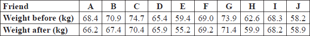
Determine unbiased estimates of the mean and variance of the loss in weight achieved over the month by people using this diet.[5]


b.(i)     State suitable hypotheses for testing whether or not this diet causes a mean loss in weight.

(ii)     Determine the value of a suitable statistic for testing your hypotheses.

(iii)     Find the 1 % critical value for your statistic and state your conclusion.[6]

 
▶️Answer/Explanation

Markscheme

the weight losses are

2.2\(\,\,\,\,\,\)3.5\(\,\,\,\,\,\)4.3\(\,\,\,\,\,\)–0.5\(\,\,\,\,\,\)4.2\(\,\,\,\,\,\)–0.2\(\,\,\,\,\,\)2.5\(\,\,\,\,\,\)2.7\(\,\,\,\,\,\)0.1\(\,\,\,\,\,\)–0.7     (M1)(A1)

\(\sum {x = 18.1} \), \(\sum {{x^2} = 67.55} \)

UE of mean = 1.81     A1

UE of variance \( = \frac{{67.55}}{9} – \frac{{{{18.1}^2}}}{{90}} = 3.87\)     (M1)A1

Note: Accept weight losses as positive or negative. Accept unbiased estimate of mean as positive or negative.


Note: Award M1A0 for 1.97 as UE of variance.


[5 marks]

a.

(i)     \({H_0}:{\mu _d} = 0\) versus \({H_1}:{\mu _d} > 0\)     A1

Note: Accept any symbol for \({\mu _d}\)


(ii)     using t test     (M1)

\(t = \frac{{1.81}}{{\sqrt {\frac{{3.87}}{{10}}} }} = 2.91\)     A1


(iii)     DF = 9     (A1)

Note: Award this (A1) if the p-value is given as 0.00864


1% critical value = 2.82     A1

accept \({H_1}\)     R1

Note: Allow FT on final R1.


[6 marks]

b.

Examiners report

In (a), most candidates gave a correct estimate for the mean but the variance estimate was often incorrect. Some candidates who use their GDC seem to be unable to obtain the unbiased variance estimate from the numbers on the screen. The way to proceed, of course, is to realise that the larger of the two ‘standard deviations’ on offer is the square root of the unbiased estimate so that its square gives the required result. In (b), most candidates realised that the t-distribution should be used although many were awarded an arithmetic penalty for giving either t = 2.911 or the critical value = 2.821. Some candidates who used the p-value method to reach a conclusion lost a mark by omitting to give the critical value. Many candidates found part (c) difficult and although they were able to obtain t = 2.49…, they were then unable to continue to obtain the confidence interval.

a.

In (a), most candidates gave a correct estimate for the mean but the variance estimate was often incorrect. Some candidates who use their GDC seem to be unable to obtain the unbiased variance estimate from the numbers on the screen. The way to proceed, of course, is to realise that the larger of the two ‘standard deviations’ on offer is the square root of the unbiased estimate so that its square gives the required result. In (b), most candidates realised that the t-distribution should be used although many were awarded an arithmetic penalty for giving either t = 2.911 or the critical value = 2.821. Some candidates who used the p-value method to reach a conclusion lost a mark by omitting to give the critical value. Many candidates found part (c) difficult and although they were able to obtain t = 2.49…, they were then unable to continue to obtain the confidence interval.

b.

Question

A baker produces loaves of bread that he claims weigh on average 800 g each. Many customers believe the average weight of his loaves is less than this. A food inspector visits the bakery and weighs a random sample of 10 loaves, with the following results, in grams:

783, 802, 804, 785, 810, 805, 789, 781, 800, 791.

Assume that these results are taken from a normal distribution.

a.Determine unbiased estimates for the mean and variance of the distribution.[3]


b.In spite of these results the baker insists that his claim is correct.

Stating appropriate hypotheses, test the baker’s claim at the 10 % level of significance.[7]

 
▶️Answer/Explanation

Markscheme

unbiased estimate of the mean: 795 (grams)     A1

unbiased estimate of the variance: 108 \((gram{s^2})\)     (M1)A1

[3 marks]

a.

null hypothesis \({H_0}:\mu  = 800\)     A1

alternative hypothesis \({H_1}:\mu  < 800\)     A1

using 1-tailed t-test     (M1)

EITHER

p = 0.0812…     A3

OR

with 9 degrees of freedom     (A1)

\({t_{calc}} = \frac{{\sqrt {10} (795 – 800)}}{{\sqrt {108} }} = – 1.521\)     A1

\({t_{crit}} = – 1.383\)     A1 

Note: Accept 2sf intermediate results.


THEN

so the baker’s claim is rejected     R1 

Note: Accept “reject \({H_0}\) ” provided \({H_0}\) has been correctly stated.


Note: FT for the final R1.


[7 marks]

b.

Examiners report

A successful question for many candidates. A few candidates did not read the question and adopted a 2-tailed test.

a.

A successful question for many candidates. A few candidates did not read the question and adopted a 2-tailed test.

b.

Question

The random variable X is normally distributed with unknown mean \(\mu \) and unknown variance \({\sigma ^2}\). A random sample of 20 observations on X gave the following results.

\[\sum {x = 280,{\text{ }}\sum {{x^2} = 3977.57} } \]

a.Find unbiased estimates of \(\mu \) and \({\sigma ^2}\).[3]


b.Determine a 95 % confidence interval for \(\mu \).[3]


c.Given the hypotheses

\[{{\text{H}}_0}:\mu  = 15;{\text{ }}{{\text{H}}_1}:\mu  \ne 15,\]

find the p-value of the above results and state your conclusion at the 1 % significance level.[4]

 
▶️Answer/Explanation

Markscheme

\(\bar x = 14\)     A1

\(s_{n – 1}^2 = \frac{{3977.57}}{{19}} – \frac{{{{280}^2}}}{{380}}\)     (M1)

\( = 3.03\)     A1

[3 marks]

Note: Accept any notation for these estimates including \(\mu \) and \({\sigma ^2}\).

Note: Award M0A0 for division by 20.

a.

the 95% confidence limits are

\(\bar x \pm t\sqrt {\frac{{s_{n – 1}^2}}{n}} \)     (M1)

Note: Award M0 for use of z.


ie, \(14 \pm 2.093\sqrt {\frac{{3.03}}{{20}}} \)     (A1)

Note:FT their mean and variance from (a).


giving [13.2, 14.8]     A1

Note: Accept any answers which round to 13.2 and 14.8.


[3 marks]

b.

Use of t-statistic \(\left( { = \frac{{14 – 15}}{{\sqrt {\frac{{3.03}}{{20}}} }}} \right)\)     (M1)

Note:FT their mean and variance from (a).


Note: Award M0 for use of z.


Note: Accept \(\frac{{15 – 14}}{{\sqrt {\frac{{3.03}}{{20}}} }}\).


\( = – 2.569 \ldots \)     (A1)

Note: Accept \(2.569 \ldots \)


\(p{\text{ – value}} = 0.009392 \ldots  \times 2 = 0.0188\)     A1

Note: Accept any answer that rounds to 0.019.


Note: Award (M1)(A1)A0 for any answer that rounds to 0.0094.


insufficient evidence to reject \({{\text{H}}_0}\) (or equivalent, eg accept \({{\text{H}}_0}\) or reject \({{\text{H}}_1}\))     R1

Note:FT on their p-value.


[4 marks]

c.

Examiners report

In (a), most candidates estimated the mean correctly although many candidates failed to obtain a correct unbiased estimate for the variance. The most common error was to divide \(\sum {{x^2}} \) by \(20\) instead of \(19\). For some candidates, this was not a costly error since we followed through their variance into (b) and (c).

a.

In (b) and (c), since the variance was estimated, the confidence interval and test should have been carried out using the t-distribution. It was extremely disappointing to note that many candidates found a Z-interval and used a Z-test and no marks were awarded for doing this. Candidates should be aware that having to estimate the variance is a signpost pointing towards the t-distribution.

b.

In (b) and (c), since the variance was estimated, the confidence interval and test should have been carried out using the t-distribution. It was extremely disappointing to note that many candidates found a Z-interval and used a Z-test and no marks were awarded for doing this. Candidates should be aware that having to estimate the variance is a signpost pointing towards the t-distribution.

c.

Question

(a)     Consider the random variable \(X\) for which \({\text{E}}(X) = a\lambda  + b\), where \(a\) and \(b\)are constants and \(\lambda \) is a parameter.

Show that \(\frac{{X – b}}{a}\) is an unbiased estimator for \(\lambda \).

(b)     The continuous random variable Y has probability density function

\(f(y) = \left\{ \begin{array}{r}{\textstyle{2 \over 9}}(3 + y – \lambda ),\\0,\end{array} \right.\begin{array}{*{20}{l}}{{\rm{ for}}\, \lambda  – 3 \le y \le \lambda }\\{{\rm{ otherwise}}}\end{array}\)

where \(\lambda \) is a parameter.

          (i)     Verify that \(f(y)\) is a probability density function for all values of \(\lambda \).

          (ii)     Determine \({\text{E}}(Y)\).

          (iii)     Write down an unbiased estimator for \(\lambda \).

▶️Answer/Explanation

Markscheme

(a)     \({\text{E}}\left( {\frac{{X – b}}{a}} \right) = \frac{{a\lambda  + b – b}}{a}\)     M1A1

\( = \lambda \)     A1

(Therefore \(\frac{{X – b}}{a}\) is an unbiased estimator for \(\lambda \))     AG

[3 marks]


(b)     (i)     \(f(y) \geqslant 0\)     R1

Note:     Only award R1 if this statement is made explicitly.

          recognition or showing that integral of f is 1 (seen anywhere) R1

          EITHER

          \(\int_{\lambda  – 3}^\lambda  {\frac{2}{9}(3 + y – \lambda ){\text{d}}y} \)     M1

          \( = \frac{2}{9}\left[ {(3 – \lambda )y + \frac{1}{2}{y^2}} \right]_{\lambda  – 3}^\lambda \)     A1

          \( = \frac{2}{9}\left( {\lambda (3 – \lambda ) + \frac{1}{2}{\lambda ^2} – (3 – \lambda )(\lambda  – 3) – \frac{1}{2}{{(\lambda  – 3)}^2}} \right)\) or equivalent     A1

          \( = 1\)

          OR

          the graph of the probability density is a triangle with base length 3 and height \(\frac{2}{3}\)     M1A1

          its area is therefore \(\frac{1}{2} \times 3 \times \frac{2}{3}\)     A1

          \( = 1\)

          (ii)     \({\text{E}}(Y) = \int_{\lambda  – 3}^\lambda  {\frac{2}{9}y(3 + y – \lambda ){\text{d}}y} \)     M1

          \( = \frac{2}{9}\left[ {(3 – \lambda )\frac{1}{2}{y^2} + \frac{1}{3}{y^3}} \right]_{\lambda  – 3}^\lambda \)     A1

          \( = \frac{2}{9}\left( {(3 – \lambda )\frac{1}{2}\left( {{\lambda ^2} – {{(\lambda  – 3)}^2}} \right) + \frac{1}{3}\left( {{\lambda ^3} – {{(\lambda  – 3)}^3}} \right)} \right)\)     M1

          \( = \lambda  – 1\)     A1A1


Note:     Award 3 marks for noting that the mean is \(\frac{2}{3}{\text{rds}}\) the way along the base and then A1A1 for \(\lambda  – 1\).

Note:     Award A1 for \(\lambda \) and A1 for –1.

          (iii)     unbiased estimator: \(Y + 1\)     A1

Note:     Accept \(\bar Y + 1\).

     Follow through their \({\text{E}}(Y)\) if linear.

[11 marks]


Total [14 marks]

Examiners report

[N/A]

Question

a.The discrete random variable X has the following probability distribution, where \(0 < \theta  < \frac{1}{3}\).


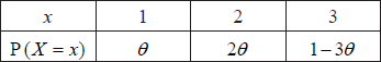
Determine \({\text{E}}(X)\) and show that \({\text{Var}}(X) = 6\theta – 16{\theta ^2}\).[4]


b.In order to estimate \(\theta \), a random sample of n observations is obtained from the distribution of X .

(i)     Given that \({\bar X}\) denotes the mean of this sample, show that

\[{{\hat \theta }_1} = \frac{{3 – \bar X}}{4}\]

is an unbiased estimator for \(\theta \) and write down an expression for the variance of \({{\hat \theta }_1}\) in terms of n and \(\theta \).

(ii)     Let Y denote the number of observations that are equal to 1 in the sample. Show that Y has the binomial distribution \({\text{B}}(n,{\text{ }}\theta )\) and deduce that \({{\hat \theta }_2} = \frac{Y}{n}\) is another unbiased estimator for \(\theta \). Obtain an expression for the variance of \({{\hat \theta }_2}\).

(iii)     Show that \({\text{Var}}({{\hat \theta }_1}) < {\text{Var}}({{\hat \theta }_2})\) and state, with a reason, which is the more efficient estimator, \({{\hat \theta }_1}\) or \({{\hat \theta }_2}\).[10]

 
▶️Answer/Explanation

Markscheme

\({\text{E}}(X) = 1 \times \theta + 2 \times 2\theta + 3(1 – 3\theta ) = 3 – 4\theta \)     M1A1

\({\text{Var}}(X) = 1 \times \theta + 4 \times 2\theta + 9(1 – 3\theta ) – {(3 – 4\theta )^2}\)     M1A1

\( = 6\theta – 16{\theta ^2}\)     AG

[4 marks]

a.

(i)     \({\text{E}}({\hat \theta _1}) = \frac{{3 – {\text{E}}(\bar X)}}{4} = \frac{{3 – (3 – 4\theta )}}{4} = \theta \)     M1A1

so \({\hat \theta _1}\) is an unbiased estimator of \(\theta \)     AG

\({\text{Var}}({{\hat \theta }_1}) = \frac{{6\theta  – 16{\theta ^2}}}{{16n}}\)     A1


(ii)     each of the n observed values has a probability \(\theta \) of having the value 1     R1

so \(Y \sim {\text{B}}(n,{\text{ }}\theta )\)     AG

\({\text{E}}({{\hat \theta }_2}) = \frac{{{\text{E}}(Y)}}{n} = \frac{{n\theta }}{n} = \theta \)     A1

\({\text{Var}}({{\hat \theta }_2}) = \frac{{n\theta (1 – \theta )}}{{{n^2}}} = \frac{{\theta (1 – \theta )}}{n}\)     M1A1


(iii)     \({\text{Var}}({{\hat \theta }_1}) – {\text{Var}}({{\hat \theta }_2}) = \frac{{6\theta  – 16{\theta ^2} – 16\theta  + 16{\theta ^2}}}{{16n}}\)     M1

\( = \frac{{ – 10\theta }}{{16n}} < 0\)     A1

\({{\hat \theta }_1}\) is the more efficient estimator since it has the smaller variance     R1

[10 marks]

b.

Examiners report

[N/A]

a.

[N/A]

b.
Scroll to Top