Download IITian Academy App for accessing Online Mock Tests and More..

Question
A curve that passes through the point (1, 2) is defined by the differential equation
\[\frac{{{\text{d}}y}}{{{\text{d}}x}} = 2x(1 + {x^2} – y){\text{ }}.\]
(a) (i) Use Euler’s method to get an approximate value of y when x = 1.3 , taking steps of 0.1. Show intermediate steps to four decimal places in a table.
(ii) How can a more accurate answer be obtained using Euler’s method?
(b) Solve the differential equation giving your answer in the form y = f(x) .
Answer/Explanation
Markscheme
(a)
(i) \(\frac{{{\text{d}}y}}{{{\text{d}}x}} = 2x(1 + {x^2} – y)\)
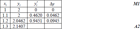
Note: Award A2 for complete table.
Award A1 for a reasonable attempt.
\(f(1.3) = 2.14\,\,\,\,\,{\text{(accept 2.141)}}\) A1
(ii) Decrease the step size A1
[5 marks]
(b) \(\frac{{{\text{d}}y}}{{{\text{d}}x}} = 2x(1 + {x^2} – y)\)
\(\frac{{{\text{d}}y}}{{{\text{d}}x}} + 2xy = 2x(1 + {x^2})\) M1
Integrating factor is \({{\text{e}}^{\int {2x{\text{d}}x} }} = {{\text{e}}^{{x^2}}}\) M1A1
So, \({{\text{e}}^{{x^2}}}y = \int {(2x} {{\text{e}}^{{x^2}}} + 2x{{\text{e}}^{{x^2}}}{x^2}){\text{d}}x\) A1
\( = {{\text{e}}^{{x^2}}} + {x^2}{{\text{e}}^{{x^2}}} – \int {2x{{\text{e}}^{{x^2}}}{\text{d}}x} \) M1A1
\( = {{\text{e}}^{{x^2}}} + {x^2}{{\text{e}}^{{x^2}}} – {{\text{e}}^{{x^2}}} + k\)
\( = {x^2}{{\text{e}}^{{x^2}}} + k\) A1
\(y = {x^2} + k{{\text{e}}^{ – {x^2}}}\)
\(x = 1,{\text{ }}y = 2 \to 2 = 1 + k{{\text{e}}^{ – 1}}\) M1
\(k = {\text{e}}\)
\(y = {x^2} + {{\text{e}}^{1 – {x^2}}}\) A1
[9 marks]
Total [14 marks]
Examiners report
Some incomplete tables spoiled what were often otherwise good solutions. Although the intermediate steps were asked to four decimal places the answer was not and the usual degree of IB accuracy was expected.
Some candidates surprisingly could not solve what was a fairly easy differential equation in part (b).
Question
Consider the differential equation \(\frac{{{\text{d}}y}}{{{\text{d}}x}} = \frac{{{y^2} + {x^2}}}{{2{x^2}}}\) for which y = −1 when x = 1.
(a) Use Euler’s method with a step length of 0.25 to find an estimate for the value of y when x = 2 .
(b) (i) Solve the differential equation giving your answer in the form \(y = f(x)\) .
(ii) Find the value of y when x = 2 .
Answer/Explanation
Markscheme
(a) Using an increment of 0.25 in the x-values A1
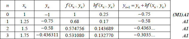
Note: The A1 marks are awarded for final column.
\( \Rightarrow y(2) \approx – 0.304\) A1
[7 marks]
(b) (i) let y = vx M1
\( \Rightarrow \frac{{{\text{d}}y}}{{{\text{d}}x}} = v + x\frac{{{\text{d}}v}}{{{\text{d}}x}}\) (A1)
\( \Rightarrow v + x\frac{{{\text{d}}v}}{{{\text{d}}x}} = \frac{{{v^2}{x^2} + {x^2}}}{{2{x^2}}}\) (M1)
\( \Rightarrow x\frac{{{\text{d}}v}}{{{\text{d}}x}} = \frac{{1 – 2v + {v^2}}}{2}\) (A1)
\( \Rightarrow x\frac{{{\text{d}}v}}{{{\text{d}}x}} = \frac{{{{(1 – v)}^2}}}{2}\) A1
\( \Rightarrow \int {\frac{2}{{{{(1 – v)}^2}}}{\text{d}}v = \int {\frac{1}{x}{\text{d}}x} } \) M1
\( \Rightarrow 2{(1 – v)^{ – 1}} = \ln x + c\) A1A1
\( \Rightarrow \frac{2}{{1 – \frac{y}{x}}} = \ln x + c\)
when \(x = 1,{\text{ }}y = – 1 \Rightarrow c = 1\) M1A1
\( \Rightarrow \frac{{2x}}{{x – y}} = \ln x + 1\)
\( \Rightarrow y = x – \frac{{2x}}{{1 + \ln x}}{\text{ }}\left( { = \frac{{x\ln x – x}}{{1 + \ln x}}} \right)\) M1A1
(ii) when \(x = 2,{\text{ }}y = – 0.362\,\,\,\,\,\left( {{\text{accept 2}} – \frac{4}{{1 + \ln 2}}} \right)\) A1
[13 marks]
Total [20 marks]
Examiners report
Part (a) was well done by many candidates, but a number were penalised for not using a sufficient number of significant figures. Part (b) was started by the majority of candidates, but only the better candidates were able to reach the end. Many were unable to complete the question correctly because they did not know what to do with the substitution y = vx and because of arithmetic errors and algebraic errors.
Question
Given that \(\frac{{{\text{d}}y}}{{{\text{d}}x}} – 2{y^2} = {{\text{e}}^x}\) and y = 1 when x = 0, use Euler’s method with a step length of 0.1 to find an approximation for the value of y when x = 0.4. Give all intermediate values with maximum possible accuracy.
Answer/Explanation
Markscheme
\(\frac{{{\text{d}}y}}{{{\text{d}}x}} = {{\text{e}}^x} + 2{y^2}\) (A1)
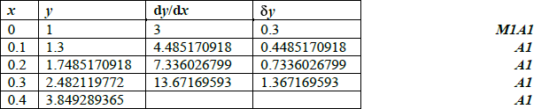
required approximation = 3.85 A1
[8 marks]
Examiners report
Most candidates seemed familiar with Euler’s method. The most common way of losing marks was either to round intermediate answers to insufficient accuracy despite the advice in the question or simply to make an arithmetic error. Many candidates were given an accuracy penalty for not rounding their answer to three significant figures.
Question
Consider the differential equation \(\frac{{{\text{d}}y}}{{{\text{d}}x}} = {x^2} + {y^2}\) where y =1 when x = 0 .
Use Euler’s method with step length 0.1 to find an approximate value of y when x = 0.4.
Write down, giving a reason, whether your approximate value for y is greater than or less than the actual value of y .
Answer/Explanation
Markscheme
use of \(y \to y + h\frac{{{\text{d}}y}}{{{\text{d}}x}}\) (M1)
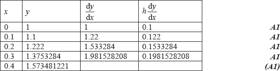
approximate value of y = 1.57 A1
Note: Accept values in the tables correct to 3 significant figures.
[7 marks]
the approximate value is less than the actual value because it is assumed that \(\frac{{{\text{d}}y}}{{{\text{d}}x}}\) remains constant throughout each interval whereas it is actually an increasing function R1
[1 mark]
Examiners report
Most candidates were familiar with Euler’s method. The most common way of losing marks was either to round intermediate answers to insufficient accuracy or simply to make an arithmetic error. Many candidates were given an accuracy penalty for not rounding their answer to three significant figures. Few candidates were able to answer (b) correctly with most believing incorrectly that the step length was a relevant factor.
Most candidates were familiar with Euler’s method. The most common way of losing marks was either to round intermediate answers to insufficient accuracy or simply to make an arithmetic error. Many candidates were given an accuracy penalty for not rounding their answer to three significant figures. Few candidates were able to answer (b) correctly with most believing incorrectly that the step length was a relevant factor.
Question
A particle moves in a straight line with velocity v metres per second. At any time t seconds, \(0 \leqslant t < \frac{{3\pi }}{4}\), the velocity is given by the differential equation \(\frac{{{\text{d}}v}}{{{\text{d}}t}} + {v^2} + 1 = 0\) .
It is also given that v = 1 when t = 0 .
Find an expression for v in terms of t .
Sketch the graph of v against t , clearly showing the coordinates of any intercepts, and the equations of any asymptotes.
(i) Write down the time T at which the velocity is zero.
(ii) Find the distance travelled in the interval [0, T] .
Find an expression for s , the displacement, in terms of t , given that s = 0 when t = 0 .
Hence, or otherwise, show that \(s = \frac{1}{2}\ln \frac{2}{{1 + {v^2}}}\).
Answer/Explanation
Markscheme
\(\frac{{{\text{d}}v}}{{{\text{d}}t}} = – {v^2} – 1\)
attempt to separate the variables M1
\(\int {\frac{1}{{1 + {v^2}}}{\text{d}}v = \int { – 1{\text{d}}t} } \) A1
\(\arctan v = – t + k\) A1A1
Note: Do not penalize the lack of constant at this stage.
when t = 0, v = 1 M1
\( \Rightarrow k = \arctan 1 = \left( {\frac{\pi }{4}} \right) = (45^\circ )\) A1
\( \Rightarrow v = \tan \left( {\frac{\pi }{4} – t} \right)\) A1
[7 marks]
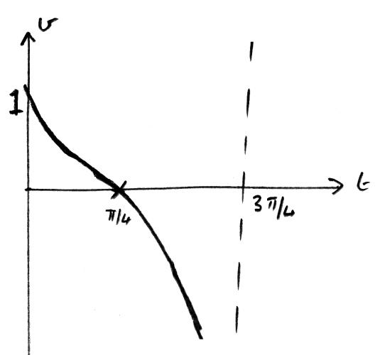 A1A1A1
Note: Award A1 for general shape,
A1 for asymptote,
A1 for correct t and v intercept.
Note: Do not penalise if a larger domain is used.
[3 marks]
(i) \(T = \frac{\pi }{4}\) A1
(ii) area under curve \( = \int_0^{\frac{\pi }{4}} {\tan \left( {\frac{\pi }{4} – t} \right){\text{d}}t} \) (M1)
\( = 0.347\left( { = \frac{1}{2}\ln 2} \right)\) A1
[3 marks]
\(v = \tan \left( {\frac{\pi }{4} – t} \right)\)
\(s = \int {\tan \left( {\frac{\pi }{4} – t} \right){\text{d}}t} \) M1
\(\int {\frac{{\sin \left( {\frac{\pi }{4} – t} \right)}}{{\cos \left( {\frac{\pi }{4} – t} \right)}}} {\text{ d}}t\) (M1)
\( = \ln \cos \left( {\frac{\pi }{4} – t} \right) + k\) A1
when \(t = 0,{\text{ }}s = 0\)
\(k = – \ln \cos \frac{\pi }{4}\) A1
\(s = \ln \cos \left( {\frac{\pi }{4} – t} \right) – \ln \cos \frac{\pi }{4}\left( { = \ln \left[ {\sqrt 2 \cos \left( {\frac{\pi }{4} – t} \right)} \right]} \right)\) A1
[5 marks]
METHOD 1
\(\frac{\pi }{4} – t = \arctan v\) M1
\(t = \frac{\pi }{4} – \arctan v\)
\(s = \ln \left[ {\sqrt 2 \cos \left( {\frac{\pi }{4} – \frac{\pi }{4} + \arctan v} \right)} \right]\)
\(s = \ln \left[ {\sqrt 2 \cos (\arctan v)} \right]\) M1A1
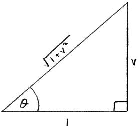
\(s = \ln \left[ {\sqrt 2 \cos \left( {\arccos \frac{1}{{\sqrt {1 + {v^2}} }}} \right)} \right]\) A1
\( = \ln \frac{{\sqrt 2 }}{{\sqrt {1 + {v^2}} }}\)
\( = \frac{1}{2}\ln \frac{2}{{1 + {v^2}}}\) AG
METHOD 2
\(s = \ln \cos \left( {\frac{\pi }{4} – t} \right) – \ln \cos \frac{\pi }{4}\)
\( = – \ln \sec \left( {\frac{\pi }{4} – t} \right) – \ln \cos \frac{\pi }{4}\) M1
\( = – \ln \sqrt {1 + {{\tan }^2}\left( {\frac{\pi }{4} – t} \right)} – \ln \cos \frac{\pi }{4}\) M1
\( = – \ln \sqrt {1 + {v^2}} – \ln \cos \frac{\pi }{4}\) A1
\( = \ln \frac{1}{{\sqrt {1 + {v^2}} }} + \ln \sqrt 2 \) A1
\( = \frac{1}{2}\ln \frac{2}{{1 + {v^2}}}\) AG
METHOD 3
\(v\frac{{dv}}{{ds}} = – {v^2} – 1\) M1
\(\int {\frac{v}{{{v^2} + 1}}dv = – \int {1ds} } \) M1
\(\frac{1}{2}\ln ({v^2} + 1) = – s + k\) A1
when \(s = 0\,,{\text{ }}t = 0 \Rightarrow v = 1\)
\( \Rightarrow k = \frac{1}{2}\ln 2\) A1
\( \Rightarrow s = \frac{1}{2}\ln \frac{2}{{1 + {v^2}}}\) AG
[4 marks]
Examiners report
This proved to be the most challenging question in section B with only a very small number of candidates producing fully correct answers. Many candidates did not realise that part (a) was a differential equation that needed to be solved using a method of separating the variables. Without this, further progress with the question was difficult. For those who did succeed in part (a), parts (b) and (c) were relatively well done. For the minority of candidates who attempted parts (d) and (e) only the best recognised the correct methods.
This proved to be the most challenging question in section B with only a very small number of candidates producing fully correct answers. Many candidates did not realise that part (a) was a differential equation that needed to be solved using a method of separating the variables. Without this, further progress with the question was difficult. For those who did succeed in part (a), parts (b) and (c) were relatively well done. For the minority of candidates who attempted parts (d) and (e) only the best recognised the correct methods.
This proved to be the most challenging question in section B with only a very small number of candidates producing fully correct answers. Many candidates did not realise that part (a) was a differential equation that needed to be solved using a method of separating the variables. Without this, further progress with the question was difficult. For those who did succeed in part (a), parts (b) and (c) were relatively well done. For the minority of candidates who attempted parts (d) and (e) only the best recognised the correct methods.
This proved to be the most challenging question in section B with only a very small number of candidates producing fully correct answers. Many candidates did not realise that part (a) was a differential equation that needed to be solved using a method of separating the variables. Without this, further progress with the question was difficult. For those who did succeed in part (a), parts (b) and (c) were relatively well done. For the minority of candidates who attempted parts (d) and (e) only the best recognised the correct methods.
This proved to be the most challenging question in section B with only a very small number of candidates producing fully correct answers. Many candidates did not realise that part (a) was a differential equation that needed to be solved using a method of separating the variables. Without this, further progress with the question was difficult. For those who did succeed in part (a), parts (b) and (c) were relatively well done. For the minority of candidates who attempted parts (d) and (e) only the best recognised the correct methods.
Question
Consider the differential equation \(\frac{{{\text{d}}y}}{{{\text{d}}x}} = f(x,{\text{ }}y)\) where \(f(x,{\text{ }}y) = y – 2x\).
Sketch, on one diagram, the four isoclines corresponding to \(f(x,{\text{ }}y) = k\) where \(k\) takes the values \(-1\), \(-0.5\), \(0\) and \(1\). Indicate clearly where each isocline crosses the \(y\) axis.
A curve, \(C\), passes through the point \((0,1)\) and satisfies the differential equation above.
Sketch \(C\) on your diagram.
A curve, \(C\), passes through the point \((0,1)\) and satisfies the differential equation above.
State a particular relationship between the isocline \(f(x,{\text{ }}y) = – 0.5\) and the curve \(C\), at their point of intersection.
A curve, \(C\), passes through the point \((0,1)\) and satisfies the differential equation above.
Use Euler’s method with a step interval of \(0.1\) to find an approximate value for \(y\) on \(C\), when \(x = 0{\text{.}}5\).
Answer/Explanation
Markscheme
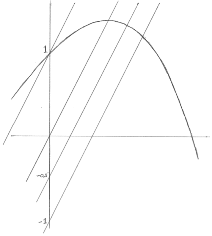
A1 for 4 parallel straight lines with a positive gradient A1
A1 for correct \(y\) intercepts A1
[2 marks]

A1 for passing through \((0,1)\) with positive gradient less than \(2\)
A1 for stationary point on \(y = 2x\)
A1 for negative gradient on both of the other \(2\) isoclines A1A1A1
[3 marks]
The isocline is perpendicular to \(C\) R1
[1 mark]
\({y_{n + 1}} = {y_n} + 0.1({y_n} – 2{x_n})\;\;\;( = 1.1{y_n} – 0.2{x_n})\) (M1)(A1)
Note: Also award M1A1 if no formula seen but \({y_2}\) is correct.
\({y_0} = 1,{\text{ }}{y_1} = 1.1,{\text{ }}{y_2} = 1.19,{\text{ }}{y_3} = 1.269,{\text{ }}{y_4} = 1.3359\) (M1)
\({y_5} = 1.39{\text{ to 3sf}}\) A1
Note: M1 is for repeated use of their formula, with steps of \(0.1\).
Note: Accept \(1.39\) or \(1.4\) only.
[4 marks]
Total [10 marks]
Examiners report
Some candidates ignored the instruction to prove from first principles and instead used standard differentiation. Some candidates also only found a derivative from one side.
Parts (b) and (c) were attempted by very few candidates. Few recognized that the gradient of the curve had to equal the value of \(k\) on the isocline.
Parts (b) and (c) were attempted by very few candidates. Few recognized that the gradient of the curve had to equal the value of \(k\) on the isocline.
Those candidates who knew the method managed to score well on this part. On most calculators a short program can be written in the exam to make Euler’s method very quick. Quite a few candidates were losing time by calculating and writing out many intermediate values, rather than just the \(x\) and\(y\) values.
Question
The curves \(y = f(x)\) and \(y = g(x)\) both pass through the point \((1,{\text{ }}0)\) and are defined by the differential equations \(\frac{{{\text{d}}y}}{{{\text{d}}x}} = x – {y^2}\) and \(\frac{{{\text{d}}y}}{{{\text{d}}x}} = y – {x^2}\) respectively.
Show that the tangent to the curve \(y = f(x)\) at the point \((1,{\text{ }}0)\) is normal to the curve \(y = g(x)\) at the point \((1,{\text{ }}0)\).
Find \(g(x)\).
Use Euler’s method with steps of \(0.2\) to estimate \(f(2)\) to \(5\) decimal places.
Explain why \(y = f(x)\) cannot cross the isocline \(x – {y^2} = 0\), for \(x > 1\).
(i) Sketch the isoclines \(x – {y^2} = – 2,{\text{ }}0,{\text{ }}1\).
(ii) On the same set of axes, sketch the graph of \(f\).
Answer/Explanation
Markscheme
gradient of \(f\) at \((1,{\text{ }}0)\) is \(1 – {0^2} = 1\) and the gradient of \(g\) at \((1,{\text{ }}0)\) is \(0 – {1^2} = – 1\) A1
so gradient of normal is \(1\) A1
= Gradient of the tangent of \(f\) at \((1,{\text{ }}0)\) AG
[2 marks]
\(\frac{{{\text{d}}y}}{{{\text{d}}x}} – y = – {x^2}\)
integrating factor is \({{\text{e}}^{\int { – 1{\text{d}}x} }} = {{\text{e}}^{ – x}}\) M1
\(y{{\text{e}}^{ – x}} = \int { – {x^2}{{\text{e}}^{ – x}}{\text{d}}x} \) A1
\( = {x^2}{{\text{e}}^{ – x}} – \int {2x{{\text{e}}^{ – x}}{\text{d}}x} \) M1
\( = {x^2}{{\text{e}}^{ – x}} + 2x{{\text{e}}^{ – x}} – \int {2{{\text{e}}^{ – x}}{\text{d}}x} \)
\( = {x^2}{{\text{e}}^{ – x}} + 2x{{\text{e}}^{ – x}} + 2{{\text{e}}^{ – x}} + c\) A1
Note: Condone missing \( + c\) at this stage.
\( \Rightarrow g(x) = {x^2} + 2x + 2 + c{{\text{e}}^x}\)
\(g(1) = 0 \Rightarrow c = – \frac{5}{{\text{e}}}\) M1
\( \Rightarrow g(x) = {x^2} + 2x + 2 – 5{{\text{e}}^{x – 1}}\) A1
[6 marks]
use of \({y_{n + 1}} = {y_n} + hf'({x_n},{\text{ }}{y_n})\) (M1)
\({x_0} = 1,{\text{ }}{y_0} = 0\)
\({x_1} = 1.2,{\text{ }}{y_1} = 0.2\) A1
\({x_2} = 1.4,{\text{ }}{y_2} = 0.432\) (M1)(A1)
\({x_3} = 1.6,{\text{ }}{y_3} = 0.67467 \ldots \)
\({x_4} = 1.8,{\text{ }}{y_4} = 0.90363 \ldots \)
\({x_5} = 2,{\text{ }}{y_5} = 1.1003255 \ldots \)
answer \( = 1.10033\) A1 N3
Note: Award A0 or N1 if \(1.10\) given as answer.
[5 marks]
at the point \((1,{\text{ }}0)\), the gradient of \(f\) is positive so the graph of \(f\) passes into the first quadrant for \(x > 1\)
in the first quadrant below the curve \(x – {y^2} = 0\) the gradient of \(f\) is positive R1
the curve \(x – {y^2} = 0\) has positive gradient in the first quadrant R1
if \(f\) were to reach \(x – {y^2} = 0\) it would have gradient of zero, and therefore would not cross R1
[3 marks]
(i) and (ii)
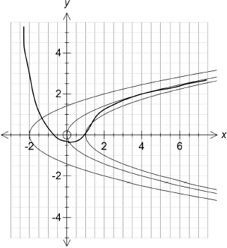 A4
A4
Note: Award A1 for 3 correct isoclines.
Award A1 for \(f\) not reaching \(x – {y^2} = 0\).
Award A1 for turning point of \(f\) on \(x – {y^2} = 0\).
Award A1 for negative gradient to the left of the turning point.
Note: Award A1 for correct shape and position if curve drawn without any isoclines.
[4 marks]
Total [20 marks]
Examiners report
[N/A]
[N/A]
[N/A]
[N/A]
[N/A]